Polarizer optimization
Overview
An interesting feature of Mitsuba is its ability to account for the polarization state of light. This becomes even more powerful when combined with differentiable rendering.
This tutorial demonstrates how those two concepts can be used together to perform a simple optimization. The setup is the following: we place two linear polarization filters in front of the camera. Initially, these are rotated in such a way that all the light passes through them. The optimization process will attempt to rotate one of the filter to minimize the overall brightness of the rendered image. Indeed, it is known that rotating this filter by 90 degrees will lead to complete cancelation of the polarization state, resulting in a darker image.
More information about polarization can be found here.
🚀 You will learn how to:
Employ differentiable rendering in the context of polarized rendering
Optimize latent variables to control the rotation of an object
Reference image
As usual, let’s import the necessary libraries. For the sake of this tutorial, we already provide an XML file for the scene containing both linear polarization filter (e.g. using the polarizer BSDF).
[1]:
import drjit as dr
import mitsuba as mi

mi.set_variant('llvm_ad_rgb_polarized')

scene = mi.load_file('../scenes/polarizers.xml')
We can then perform the rendering of our initial scene. As expected, the two filters are aligned and let linearly polarized light through.
[2]:
image_init = mi.render(scene, spp=8)

mi.util.convert_to_bitmap(image_init)
[2]:

Setup optimization
As in the previous tutorial on pose estimation, we setup the optimization using a latent variable to control the rotation of the filter. This rotation angle will be used to construct a transformation matrix that will be applied to all vertices of the filter’s mesh. For convenience, we define a function that does all of this, which we will also call later during the optimization loop.
It is important to apply the rotation once before starting the optimization loop as this will bind the optimizer variable to the scene parameter. Otherwise during backpropagation the gradients wouldn’t be propagate all the way to the optimizer’s variable.
[3]:
params = mi.traverse(scene)

# Key of the scene parameter to be optimized
key = 'filter2.vertex_positions'

# Get the initial vertex positions
v_positions_init = dr.unravel(mi.Vector3f, params[key])

# Instantiate an Adam optimizer and define a latent variable `rotation`
opt = mi.ad.Adam(lr=1.0)
opt['rotation'] = mi.Float(0.0)

# Apply optimized rotation value to mesh vertices
def apply_rotation():
    transform = mi.Transform4f().rotate([0, 0, 1], opt['rotation'])
    positions_new = transform @ v_positions_init
    params[key] = dr.ravel(positions_new)
    params.update()

# Perform the first rotation to enable derivative tracking on the scene parameters
apply_rotation()
Optimization
Everything is now ready to run the optimization loop.
In the following cell we define the hyper parameters controlling our optimization loop, such as the number of iterations:
[4]:
iteration_count = 100
In this example the loss function doesn’t compare against a reference as the goal is simply to make the image darker. For this we simply use the sum of the pixel values in the rendered image.
[6]:
angles = []
losses = []

for it in range(iteration_count):
    # Perform the differentiable rendering simulation
    image = mi.render(scene, params=params, seed=it, spp=1)

    # Objective: no comparison against a reference, the goal is simply to make the image darker
    ob_val = dr.mean(image)

    # Backpropagate loss to input parameters
    dr.backward(ob_val)

    # Optimizer: take a gradient step
    opt.step()

    # Apply rotation and update the scene parameters
    apply_rotation()

    print(f"Iteration: {it:2}, rot: {opt['rotation'][0]:.4f}, loss: {ob_val}", end='\r')
    angles.append(opt['rotation'][0])
    losses.append(ob_val.array[0])

print()
print('Optimization complete!')
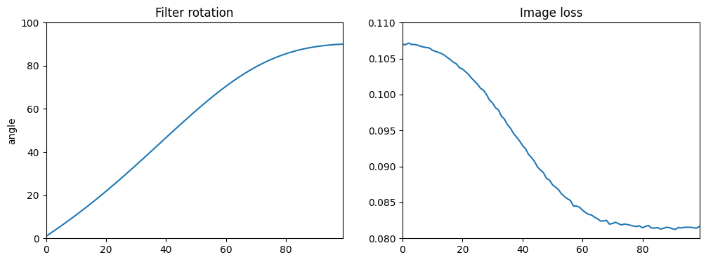
Iteration: 99, rot: 90.0260, loss: 0.0816507
Optimization complete!
Results
We can now look at the optimized scene, which appears much darker as expected.
[7]:
image_final = mi.render(scene, seed=0, spp=8)

mi.util.convert_to_bitmap(image_final)
[7]:

We plot the filter rotation and image loss accross the optimization loop.
[8]:
from matplotlib import pyplot as plt

fig, ax = plt.subplots(ncols=2, figsize=(12,4))

ax[0].plot(angles);
ax[0].set_ylabel('angle');
ax[0].set_title('Filter rotation');
ax[0].set_xlim([0, 99]);
ax[0].set_ylim([0, 100])

ax[1].plot(losses);
ax[1].set_title('Image loss')
ax[1].set_xlim([0, 99]);
ax[1].set_ylim([0.08, 0.11])

plt.show()