Choosing variants

Mitsuba 3 is a retargetable rendering system that provides a set of different system “variants” that change elementary aspects of simulation—they can for instance replace the representation of color to support monochromatic, RGB, spectral, or even polarized illumination. Similarly, the numerical representation underlying the simulation can be exchanged to perform renderings using a higher amount of precision, process many light paths at once on the GPU, or it can be mathematically differentiated to to solve inverse problems. All variants are automatically created from a single generic codebase. Each variant is associated with an identifying name that is composed of several parts:

As many as 60 different variants of the renderer are presently available, shown in the list below.

Show/hide available variants

• scalar_mono

• scalar_mono_double

• scalar_mono_polarized

• scalar_mono_polarized_double

• scalar_rgb

• scalar_rgb_double

• scalar_rgb_polarized

• scalar_rgb_polarized_double

• scalar_spectral

• scalar_spectral_double

• scalar_spectral_polarized

• scalar_spectral_polarized_double

• llvm_mono

• llvm_mono_double

• llvm_mono_polarized

• llvm_mono_polarized_double

• llvm_rgb

• llvm_rgb_double

• llvm_rgb_polarized

• llvm_rgb_polarized_double

• llvm_spectral

• llvm_spectral_double

• llvm_spectral_polarized

• llvm_spectral_polarized_double

• llvm_ad_mono

• llvm_ad_mono_double

• llvm_ad_mono_polarized

• llvm_ad_mono_polarized_double

• llvm_ad_rgb

• llvm_ad_rgb_double

• llvm_ad_rgb_polarized

• llvm_ad_rgb_polarized_double

• llvm_ad_spectral

• llvm_ad_spectral_double

• llvm_ad_spectral_polarized

• llvm_ad_spectral_polarized_double

• cuda_mono

• cuda_mono_double

• cuda_mono_polarized

• cuda_mono_polarized_double

• cuda_rgb

• cuda_rgb_double

• cuda_rgb_polarized

• cuda_rgb_polarized_double

• cuda_spectral

• cuda_spectral_double

• cuda_spectral_polarized

• cuda_spectral_polarized_double

• cuda_ad_mono

• cuda_ad_mono_double

• cuda_ad_mono_polarized

• cuda_ad_mono_polarized_double

• cuda_ad_rgb

• cuda_ad_rgb_double

• cuda_ad_rgb_polarized

• cuda_ad_rgb_polarized_double

• cuda_ad_spectral

• cuda_ad_spectral_double

• cuda_ad_spectral_polarized

• cuda_ad_spectral_polarized_double

However, when installing Mitsuba on your system with pip, only a subset of those variants will be installed.

• scalar_rgb

• scalar_spectral

• cuda_ad_rgb

• llvm_ad_rgb

This is to avoid the burden of downloading massive binaries, but those should be enough to get you started with Mitsuba 3. For advanced applications that require another variant, you will need to compile it yourself. For this please refer to the documentation on compiling the system from source.

Part 1: Computational backend

The computational backend controls how basic arithmetic operations like additions or multiplications are realized by the system. The following choices are available:

• The scalar backend performs computation on the CPU using normal floating point arithmetic similar to older versions of Mitsuba. The renderer processes individual rays at a time. This mode is the easiest to understand and therefore preferred for fixing compilation errors and debugging the renderer.

• The cuda backend offloads computation to the GPU using Dr.Jit’s just-in-time (JIT) compiler that transforms computation into CUDA kernels. Using this backend, each operation typically operates on millions of inputs at the same time. Mitsuba then becomes what is known as a wavefront path tracer and delegates ray tracing on the GPU to NVIDIA’s OptiX library. Note that this requires a relatively recent NVIDIA GPU: ideally Turing or newer. The older Pascal architecture is also supported but tends to be slower because it lacks ray tracing hardware acceleration.

• llvm: Similar to the cuda backend, the computation required to render a scene is just-in-time compiled using Dr.Jit to parallel CPU kernels that process many rays at the same time. This uses the LLVM compiler framework, which is detected and loaded at runtime. If you don’t have a NVIDIA GPU, this mode is a great alternative to the cuda backend.

An appealing aspect of the llvm and cuda modes, is that they expose vectorized Python interfaces that operate on arbitrarily large set of inputs. This means that millions of ray tracing operations or BSDF evaluations can be performed with a single Python function call, enabling efficient prototyping within Python or Jupyter notebooks without costly iteration over many elements.

Part 2: Automatic differentiation

It is possible to add the _ad suffix to enable automatic differentiation for both cuda and llvm modes. In which case the backend will furthermore propagates derivative information through the simulation, which is a crucial ingredient for solving inverse problems using rendering algorithms.

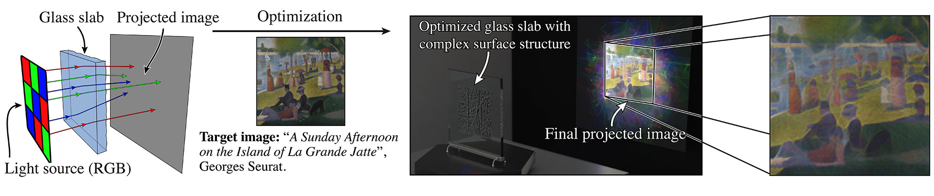
The following shows an example from [NDVZJ19]. Here, Mitsuba 3 is used to compute the height profile of a transparent glass panel that refracts red, green, and blue light in such a way as to reproduce a specified color image.

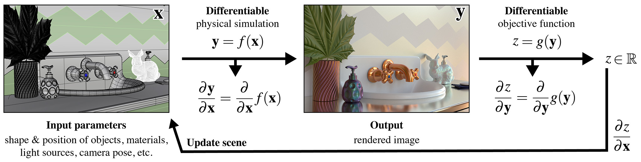
The main use case of the _ad backends is differentiable rendering, which interprets the rendering algorithm as a function \(f(\mathbf{x})\) that converts an input \(\mathbf{x}\) (the scene description) into an output \(\mathbf{y}\) (the rendering). This function \(f\) is then mathematically differentiated to obtain \(\frac{\mathrm{d}\mathbf{y}}{\mathrm{d}\mathbf{x}}\), providing a first-order approximation of how a desired change in the output \(\mathbf{y}\) (the rendering) can be achieved by changing the inputs \(\mathbf{x}\) (the scene description). Together with a differentiable objective function \(g(\mathbf{y})\) that quantifies the suitability of tentative scene parameters and a gradient-based optimization algorithm, a differentiable renderer can be used to solve complex inverse problems involving light.

The documentations provides several applied examples on differentiable and inverse rendering.

Part 3: Color representation

The next part determines how Mitsuba represents color information. The following choices are available:

• mono completely disables the concept of color, which is useful when simulating scenes that are inherently monochromatic (e.g. illumination due to a laser). This mode is great for writing testcases where color is simply not relevant. When an input scene provides color information, mono mode automatically converts it to grayscale.

• rgb mode selects an RGB-based color representation. This is a reasonable default choice and matches the typical behavior of the previous generation of Mitsuba. On the flipside, RGB mode can be a poor approximation of how color works in the real world. Please click on the following for a longer explanation.

  Issues involving RGB-based rendering (click to expand)

  Problematic aspects of RGB-based color representations: A RGB rendering algorithm frequently performs two color-related operations: component-wise addition to combine different sources of light, and component-wise multiplication of RGB color vectors to model interreflection. While addition is fine, RGB multiplication turns out to be a nonsensical operation, that can give very different answers depending on the underlying RGB color space.

  Suppose we are rendering a scene in an sRGB color space, where a green light with radiance \([0, 0, 1]\) reflects from a very green surface with albedo \([0, 0, 1]\). The component-wise multiplication \([0, 0, 1] \otimes [0, 0, 1] = [0, 0, 1]\) tells us that no light is absorbed by the surface. So good so far.

  Let’s now switch to a larger color space named Rec. 2020. That same green color is no longer at the extreme of the color gamut but lies somewhere inside.

  

  For simplicity, let’s suppose it has coordinates \([0, 0, \frac{1}{2}]\). Now, the same calculation \([0, 0, \frac{1}{2}]\otimes[0, 0, \frac{1}{2}]=[0, 0, \frac{1}{4}]\) tells us that half of the light is absorbed by the surface, which illustrates the problem with RGB multiplication. The solution to this problem is to multiply colors in the spectral domain instead.

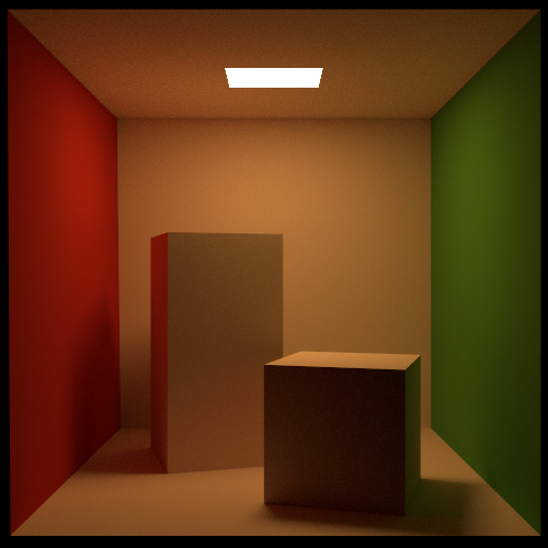
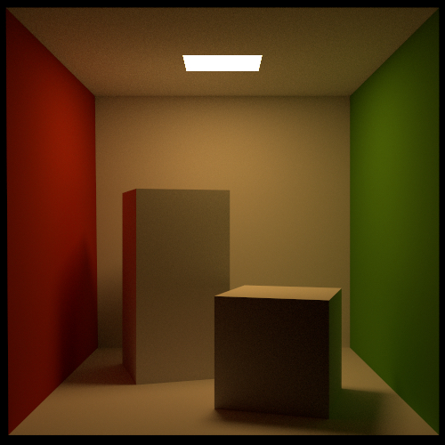
• Finally, spectral mode switches to a fully spectral color representation spanning the visible range \((360\ldots 830 \mathrm{nm})\). The wavelength domain is simply treated as yet another dimension of the space of light paths over which the rendering algorithm must integrate.

  This improves accuracy especially in scenarios where measured spectral data is available. Consider for example the two Cornell box renderings below: on the left side, the spectral reflectance data of all materials is first converted to RGB and rendered using the scalar_rgb variant, producing a deceivingly colorful image. In contrast, the scalar_spectral variant that correctly accounts for the spectral characteristics, produces a more muted coloration.

  

  RGB Mode#

  

  Spectral Mode#

  Note that Mitsuba still generates RGB output images by default even when spectral mode is active. It is also important to note that many existing Mitsuba scenes only specify RGB color information. Spectral Mitsuba can still render such scenes – in this case, it determines plausible smooth spectra corresponding to the specified RGB colors [JH19]. We also recommend taking a look at the Spectral film plugin which is able to output spectral multichannel output images.

Part 4: Polarization

If desired, Mitsuba 3 can keep track of the full polarization state of light. Polarization refers to the property that light is an electromagnetic wave that oscillates perpendicularly to the direction of travel. This oscillation can take on infinitely many different shapes—the following images show examples of horizontal and elliptical polarization.

Because humans do not perceive polarization, accounting for it is usually not necessary to render realistic images. However, polarization is easily observed using a variety of measurement devices and cameras, and it tends to provide a wealth of information about the material and shape of visible objects. For this reason, polarization is a powerful tool for solving inverse problems, and this is one of the reasons why we chose to support it in Mitsuba 3. Note that accounting for polarization comes at a cost—roughly a 1.5-2X increase in rendering time.

Inside the light transport simulation, Stokes vectors are used to parameterize the elliptical shape of the transverse oscillations, and Mueller matrices are used to compute the effect of surface scattering on the polarization [Col93]. For more details regarding the implementation of the polarized rendering modes, please refer to the Polarization section in the developer guide.

Part 5: Precision

Mitsuba 3 normally relies on single precision (32 bit) arithmetic, but double precision (64 bit) is optionally available adding the _double suffix to the variant name. We find this particularly helpful for debugging: whether or not an observed problem arises due to floating point imprecisions can normally be determined after switching to double precision. Note that Embree and OptiX don’t support double precision, hence ray-tracing operations will run in reduced (single) precision in those modes. The only way to use precision for everything including ray tracing is to render on the CPU (scalar or llvm) and disable Embree in CMake. Also note that double precision arithmetic runs with greatly reduced throughput (1/64th of FP32) on recent NVIDIA GPUs.