Testing
To run the test suite, simply invoke pytest:
pytest

# or to run a single test file
pytest src/bsdfs/tests/test_diffuse.py
If you want to skip the execution of the slower tests, you can do so by running the test suite with the following flag.
pytest -m 'not slow'
The build system also exposes a pytest target that executes setpath and
parallelizes the test execution.
ninja pytest
Testing multiple variants
The system provides a variety of Python fixture to automatically run unit tests on subsets of the available variants. Those should be passed a first argument to the test function like in the following example:
# This test will run on all available variants
def test_hello_world(variants_all):
    print(f'Hello {mi.variant()}')
    assert True
Here is the list of available fixtures:
variants_all: execute on all variants
variants_all_scalar: execute on all
scalar_*variantsvariants_all_rgb: execute on all
*_rgbvariantsvariants_all_spectral: execute on all
*_spectralvariantsvariants_all_backends_once: execute the test for at least on variant per backend
variants_all_ad_rgb: execute on all
*_ad_rgbvariantsvariants_all_ad_spectral: execute on all
*_ad_spectralvariantsvariants_any_scalar: execute on one
scalar_*variant if availablevariants_any_llvm: execute on one
llvm_*variant if availablevariants_any_cuda: execute on one
cuda_*variant if availablevariants_vec_backends_once: execute on one
cuda_*and onellvm_*variant if availablevariants_vec_backends_once_rgb: execute on one
cuda_*_rgband onellvm_*_rgbvariant if availablevariants_vec_backends_once_spectral: execute on one
cuda_*_spectraland onellvm_*_spectralvariant if availablevariants_vec_rgb: execute on
cuda_*_rgbandllvm_*_rgbvariantsvariants_vec_spectral: execute on
cuda_*_spectralandllvm_*_spectralvariants
Chi^2 tests
The mitsuba.chi2 module implements the Pearson’s chi-square test for
testing goodness of fit of a distribution to a known reference distribution.
The implementation specifically compares a Monte Carlo sampling strategy on a 2D (or lower dimensional) space against a reference distribution obtained by numerically integrating a probability density function over grid in the distribution’s parameter domain.
This is used extensively throughout the test suite to valid the implementation
of BSDFs, Emitters, and other sampling code.
It is possible to test your own sampling code in the following way:
import mitsuba as mi
mi.set_variant('llvm_rgb')

# some sampling code
def my_sample(sample):
    return mi.warp.square_to_cosine_hemisphere(sample)

# the corresponding probability density function
def my_pdf(p):
    return mi.warp.square_to_cosine_hemisphere_pdf(p)

chi2 = mi.ChiSquareTest(
    domain=mi.SphericalDomain(),
    sample_func=my_sample,
    pdf_func=my_pdf,
    sample_dim=2
)

assert chi2.run()
In case of failure, the target density and histogram were written to
chi2_data.py which can simply be run to plot the data:
python chi2_data.py
The mitsuba.chi2 module also provides a set of Adapter functions
which can be used to wrap different plugins (e.g. BSDF, Emitter, …)
in order to test them:
import mitsuba as mi
import drjit as dr

mi.set_variant('llvm_rgb')

xml = """<float name="alpha" value="0.5"/>
         <boolean name="sample_visible" value="false"/>
         <string name="distribution" value="ggx"/>
      """
wi = dr.normalize([0.2, -0.6, -0.5])
sample_func, pdf_func = mi.BSDFAdapter("roughdielectric", xml, wi=wi)

chi2 = mi.ChiSquareTest(
    domain=mi.SphericalDomain(),
    sample_func=sample_func,
    pdf_func=pdf_func,
    sample_dim=3
)

assert chi2.run()

# Forces the chi2 test to dump the plotting script (optional)
chi2._dump_tables()
Here is the figure generated by the chi2_data.py script from the example above:
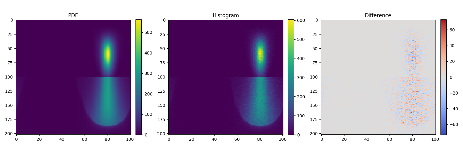
The plot on the left shows the density function generated by numerically
integrating the analytical pdf() method of a roughdielectric BSDF with
an incoming vector coming from inside. Most of the energy leaves the surface
(upper half of the plot) while some energy gets reflected back inside the
surface (lower half of the plot).
The middle plot shows the same density function but this time computed as a
histogram of sampled directions resulting from the sample() method of the
roughdielectric BSDF.
The right plot shows the difference between the two density functions. The
sampling routine of the BSDF being stochastic, it is expected to see a mix of
negative and positive values as the histogram is still noisy. The main role of
the ChiSquareTest is to decide whether the observed deviation is within the
range of random noise, or whether there are systematic biases that should lead
to a test failure.
For more information, see mitsuba.chi2.ChiSquareTest.
Rendering test suite and Z-test
On top of test unit tests, the framework implements a mechanism that automatically renders a set of test scenes and applies the Z-test to compare the resulting images and some reference images.
Those tests are really useful to reveal bugs at the interaction between the individual components of the renderer.
The test scenes are rendered using all the different enabled variants of the
renderer, ensuring for instance that the scalar_rgb renders match the
cuda_rgb renders.
To only run the rendering test suite, use the following command:
pytest src/render/tests/test_renders.py
One can easily add a scene to the resources/data/tests/scenes/ folder to add
it to the rendering test suite. Then, the missing reference images can be
generated using the following command:
python src/render/tests/test_renders.py