Object pose estimation
Overview
In this tutorial, we will show how to optimize the pose of an object while correctly accounting for the visibility discontinuities. We are going to optimize several latent variables that control the translation and rotation of the object.
In differentiable rendering, we aim to evaluate the derivative of a pixel intensity integral with respect to a scene parameter \(\pi\) as follows:
\begin{equation} \partial_\pi I(\pi) = \partial_\pi \int_P f(\textbf{x}, \pi) ~ d\textbf{x} \end{equation}
where \(\textbf{x}\) is a light path in the path space \(P\).
When the function \(f(\cdot)\) is continuous w.r.t. \(\pi\), we can move the derivative into the integral and then apply Monte Carlo integration. Under this assumption, differentiating the rendering process via automatic differentiation, as in the previous tutorials, is correct.
However, if \(f(\cdot)\) has discontinuities w.r.t. \(\pi\), direct application of automatic differentiation is not correct anymore, as it omits an integral term given by the Reynolds transport theorem. This needs to be considered when differentiating shape-related parameters (e.g., position), as the discontinuities in the visiblity function (the silhouette of the object) are then dependent on the differentiated parameter.
In the last years, several works tried to address this issue (e.g., [LADL18], [ZMY+20], [LHJ19], [BLD20], [ZRJ23], …). Mitsuba provides dedicated integrators implementing the “projective sampling”-based approach ([ZRJ23]).
direct_projective: projective sampling direct illumination integrator
prb_projective: projective sampling wth Path Replay Backpropagation (PRB) integrator
In this tutorial, we will optimize the position and rotation of a mesh in order to match a target rendering. To keep things simple, we will use the direct_projective integrator. You will learn more about this integrator in the following tutorials.
🚀 You will learn how to:
Perform an optimization with discontinuity-aware methods
Optimize latent variables to control the motion of an object
Setup
As always, let’s import drjit and mitsuba and set a differentiation-aware variant.
[1]:
import drjit as dr
import mitsuba as mi

mi.set_variant('cuda_ad_rgb', 'llvm_ad_rgb')
direct_projective and scene construction
We will rely on the direct_projective integrator for this tutorial to properly handle the visibility discontinuities in our differentiable simulation. In primal rendering, this integrator is identical to the direct integrator.
[2]:
integrator = {
    'type': 'direct_projective',
}
We create a simple scene with a bunny placed in front of a gray wall, illuminated by a spherical light.
[3]:
from mitsuba.scalar_rgb import Transform4f as T

scene = mi.load_dict({
    'type': 'scene',
    'integrator': integrator,
    'sensor':  {
        'type': 'perspective',
        'to_world': T().look_at(
                        origin=(0, 0, 2),
                        target=(0, 0, 0),
                        up=(0, 1, 0)
                    ),
        'fov': 60,
        'film': {
            'type': 'hdrfilm',
            'width': 64,
            'height': 64,
            'rfilter': { 'type': 'gaussian' },
            'sample_border': True
        },
    },
    'wall': {
        'type': 'obj',
        'filename': '../scenes/meshes/rectangle.obj',
        'to_world': T().translate([0, 0, -2]).scale(2.0),
        'face_normals': True,
        'bsdf': {
            'type': 'diffuse',
            'reflectance': { 'type': 'rgb', 'value': (0.5, 0.5, 0.5) },
        }
    },
    'bunny': {
        'type': 'ply',
        'filename': '../scenes/meshes/bunny.ply',
        'to_world': T().scale(6.5),
        'bsdf': {
            'type': 'diffuse',
            'reflectance': { 'type': 'rgb', 'value': (0.3, 0.3, 0.75) },
        },
    },
    'light': {
        'type': 'obj',
        'filename': '../scenes/meshes/sphere.obj',
        'emitter': {
            'type': 'area',
            'radiance': {'type': 'rgb', 'value': [1e3, 1e3, 1e3]}
        },
        'to_world': T().translate([2.5, 2.5, 7.0]).scale(0.25)
    }
})
Reference image
Next we generate the target rendering. We will later modify the bunny’s position and rotation to set the initial optimization state.
[4]:
img_ref = mi.render(scene, seed=0, spp=1024)

mi.util.convert_to_bitmap(img_ref)
[4]:

Optimizer and latent variables
As done in previous tutorial, we access the scene parameters using the traverse() mechanism. We then store a copy of the initial vertex positions. Those will be used later to compute the new vertex positions at every iteration, always applying a different transformation on the same base shape.
Since the vertex positions in Mesh are stored in a linear buffer (e.g., x_1, y_1, z_1, x_2, y_2, z_2, ...), we use the dr.unravel() routine to unflatten that array into a Point3f array.
[5]:
params = mi.traverse(scene)
initial_vertex_positions = dr.unravel(mi.Point3f, params['bunny.vertex_positions'])
While it would be possible to optimize the vertex positions of the bunny independently, in this example we are only going to optimize a translation and rotation parameter. This drastically constrains the optimization process, which helps with convergence.
Therefore, we instantiate an optimizer and assign two variables to it: angle and trans.
[6]:
opt = mi.ad.Adam(lr=0.025)
opt['angle'] = mi.Float(0.25)
opt['trans'] = mi.Point2f(0.1, -0.25)
From the optimizer’s point of view, those variables are the same as any other variables optimized in the previous tutorials, to the exception that when calling opt.update(), the optimizer doesn’t know how to propagate their new values to the scene parameters. This has to be done manually, and we encapsulate exactly that logic in the function defined below. More detailed explaination on this can be found
here.
After clipping the optimized variables to a proper range, this function creates a transformation object combining a translation and rotation and applies it to the vertex positions stored previously. It then flattens those new vertex positions before assigning them to the scene parameters.
[7]:
def apply_transformation(params, opt):
    opt['trans'] = dr.clip(opt['trans'], -0.5, 0.5)
    opt['angle'] = dr.clip(opt['angle'], -0.5, 0.5)

    trafo = mi.Transform4f().translate([opt['trans'].x, opt['trans'].y, 0.0]).rotate([0, 1, 0], opt['angle'] * 100.0)

    params['bunny.vertex_positions'] = dr.ravel(trafo @ initial_vertex_positions)
    params.update()
It is now time to apply our first transformation to get the bunny to its initial state before starting the optimization.
[8]:
apply_transformation(params, opt)

img_init = mi.render(scene, seed=0, spp=1024)

mi.util.convert_to_bitmap(img_init)
[8]:

In the following cell we define the hyper parameters controlling the optimization, such as the number of iterations and number of samples per pixels for the differentiable rendering simulation:
[9]:
iteration_count = 100
spp = 16
The optimization loop below is very similar to the one used in the other tutorials, except that we need to apply the transformation to update the bunny’s state and record the relation between the rendered image and the optimized parameters.
[11]:
import time
loss_hist = []
for it in range(iteration_count):
    # Apply the mesh transformation
    apply_transformation(params, opt)

    # Perform a differentiable rendering
    img = mi.render(scene, params, seed=it, spp=spp)

    # Evaluate the objective function
    loss = dr.sum(dr.square(img - img_ref)) / len(img.array)

    # Backpropagate through the rendering process
    dr.backward(loss)

    # Optimizer: take a gradient descent step
    opt.step()

    loss_hist.append(loss.array[0])
    print(f"Iteration {it:02d}: error={loss}, angle={opt['angle'][0]:.4f}, trans=[{opt['trans'].x[0]:.4f}, {opt['trans'].y[0]:.4f}]", end='\r')
Iteration 99: error=0.00266705, angle=-0.0015, trans=[-0.0013, -0.0016]
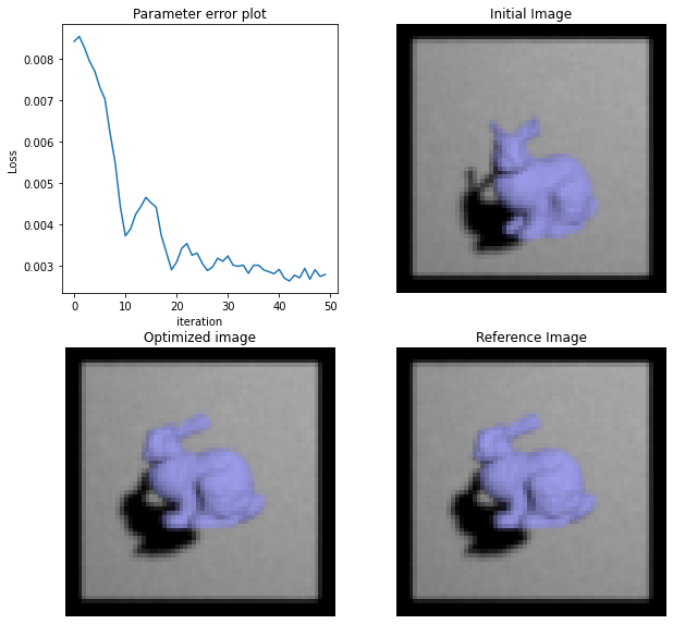
Visualizing the results
Finally, let’s visualize the results and plot the loss over iterations
[12]:
from matplotlib import pyplot as plt

fig, axs = plt.subplots(2, 2, figsize=(10, 10))

axs[0][0].plot(loss_hist)
axs[0][0].set_xlabel('iteration');
axs[0][0].set_ylabel('Loss');
axs[0][0].set_title('Parameter error plot');

axs[0][1].imshow(mi.util.convert_to_bitmap(img_init))
axs[0][1].axis('off')
axs[0][1].set_title('Initial Image')

axs[1][0].imshow(mi.util.convert_to_bitmap(mi.render(scene, spp=1024)))
axs[1][0].axis('off')
axs[1][0].set_title('Optimized image')

axs[1][1].imshow(mi.util.convert_to_bitmap(img_ref))
axs[1][1].axis('off')
axs[1][1].set_title('Reference Image');