Polarization

Introduction

The retargetable design of the Mitsuba 3 rendering system can be leveraged to optionally keep track of the full polarization state of light, meaning that it simulates the oscillations of the light’s electromagnetic wave perpendicular to its direction of travel.

Because humans do not perceive this directly, accounting for it is usually not necessary when rendering images that are intended to look realistic. However, polarization is easily observed using a variety of measurement devices and cameras and it tends to provide a wealth of information about the material and shape of visible objects. For this reason, polarization is a powerful tool for solving inverse problems, and this is one of the reasons why we chose to support it in Mitsuba 3.

Polarized rendering has been studied extensively before. A first (unidirectional) algorithm was proposed by Wilkie and Weidlich [WW12] before it was extended to bidirectional techniques in two later works [MSWK16], [JA18] by leveraging the general path space formulation [Vea98].

Polarized rendering is also implemented by the Advanced Rendering Toolkit (ART) research rendering system.

---

The first two sections of this document cover the mathematical framework behind polarization that is relevant for rendering (Section Mathematics of polarized light) as well as an in-depth description of the Fresnel equations that are important components of many reflectance models (Section Fresnel equations). Finally, Section Implementation serves as a developer guide and explains how polarization is implemented in Mitsuba 3.

Mathematics of polarized light

In this section we go over the basics behind the mathematical representation of polarized light and how it interacts with common optical elements. No prior knowledge of polarization is required for following these Sections though we only cover the contents needed for rendering applications. More thorough discussions can be found in the optics literature [Hec98], [Col93], [Col05].

Modern rendering systems are generally built on top of the radiometry framework for describing light where algorithms usually track a unit called radiance [PJH16]. This was originally based on a particle description of light and thus does not cover the effects of polarization (or other aspects of wave optics).

From the optics community, there are two commonly used frameworks to describe the polarization state of light:

1. Mueller-Stokes calculus

The polarization state (fully polarized, partially polarized, or unpolarized) is represented with a \(4 \times 1\) Stokes vector while interaction with optical elements or scattering is achieved by multiplication with \(4 \times 4\) Mueller matrices.

2. Jones calculus

This representation is simpler and uses \(2 \times 1\) and \(2 \times 2\) Jones vectors and matrices instead. They are directly related to the underlying electrical field components of the wave and can explain superpositions of waves, e.g. interference effects. However, Jones calculus can only represent fully polarized light and is therefore of limited interest for rendering applications.

Like previous work in polarized rendering [WW12], [MSWK16], [JA18], we will use the Mueller-Stokes calculus for our implementation.

Stokes vectors

Definitions

Figure 1: Illustration of the individual Stokes vector components \(\mathbf{s}_0, \mathbf{s}_1, \mathbf{s}_2, \mathbf{s}_3\) on top of the reference coordinate frame (\(\mathbf{x}, \mathbf{y}\)) where the \(\mathbf{x}\)-axis is interpreted as horizontal.

A Stokes vector is a 4-dimensional quantity \(\mathbf{s} = [\mathbf{s}_0, \mathbf{s}_1, \mathbf{s}_2, \mathbf{s}_3]^{\top}\) [[1]] which parameterizes the full polarization state of light [[2]].

• \(\mathbf{s}_0\) is equivalent to radiance normally used in physically based rendering. It measures the intensity of light but does not say anything about its polarization state.

• \(\mathbf{s}_1\) distinguishes horizontal vs. vertical linear polarization, where \(\mathbf{s}_1 = \pm 1\) stands for completely horizontally or vertically polarized light respectively.

• \(\mathbf{s}_2\) is similar to \(\mathbf{s}_1\) but distinguishes diagonal linear polarization at \(\pm 45˚\) angles, as measured from the horizontal axis.

• \(\mathbf{s}_3\) distinguishes right vs. left circular polarization, where \(\mathbf{s}_3 = \pm 1\) stands for full right or left circularly polarized light respectively.

• Physically plausible Stokes vectors need to fulfill \(\mathbf{s}_0 \geq \sqrt{\mathbf{s}_1^2 + \mathbf{s}_2^2 + \mathbf{s}_3^2}\).

A few typical examples of interesting polarization states are summarized in the following table and animations.

Description	Corresponding Stokes vector
Unpolarized light	\([1, 0, 0, 0]^{\top}\)
Horizontal linearly polarized light	\([1, 1, 0, 0]^{\top}\)
Vertical linearly polarized light	\([1, -1, 0, 0]^{\top}\)
Diagonal (+45˚) linearly polarized light	\([1, 0, 1, 0]^{\top}\)
Diagonal (-45˚) linearly polarized light	\([1, 0, -1, 0]^{\top}\)
Right circularly polarized light	\([1, 0, 0, 1]^{\top}\)
Left circularly polarized light	\([1, 0, 0, -1]^{\top}\)

Table 1 Common Stokes vector values.

Reference frames

As illustrated in Figure 1, these definitions above are only true relative to a given reference coordinate frame (\(\mathbf{x}, \mathbf{y}\)). Here, the \(\mathbf{x}\)-axis indicates what is meant with “horizontal”. As long as the frame is orthogonal to the beam of light, this is purely a matter of convention and infinitely many such frames exist. We follow the convention used in most textbooks and other sources with a right-handed coordinate system where the z-axis points along the light propagation direction like so [[3]]:

Note how we take the point of view of the “receiver” and look into the direction of the “source” of the beam to describe the Stokes vector. In particular, this also clarifies the handedness of circular polarization.

As a final example, consider Figure 2 which shows linearly polarized light in two different reference frames, resulting in two different Stokes vectors.

Figure 2: (Left) Linearly polarized light is observed in a reference frame \((\mathbf{x}, \mathbf{y})\) where the measured Stokes vector looks like horizontal polarization, \(\mathbf{s} = [1, 1, 0, 0]^{\top}\). (Right) The same beam is observed in a rotated reference frame \((\mathbf{x}', \mathbf{y}')\) where the Stokes vector looks like \(-45˚\) linear polarization, \(\mathbf{s} = [1, 0, -1, 0]^{\top}\).

---

[1]

In some sources, the notation \(\mathbf{s} = [I, Q, U, V]^{\top}\) is used instead.

[2]

Polarization should be tracked for each wavelength of light individually. In this document we mostly assume a monochromatic setting. We will revisit the spectral domain later during Section Implementation when discussion implementation details.

[3]

This is also known as the SPIE convention.

Mueller matrices

Any change of the polarization change due to interaction with some optical element or interface can be summarized as a multiplication of the corresponding Stokes vector with a Mueller matrix \(\mathbf{M} \in \mathbb{R}^{4x4}\). After the interaction, the incident (\(\mathbf{s}_{\text{in}}\)) and outgoing (\(\mathbf{s}_{\text{out}}\)) Stokes vectors are related by

(1)\[ \mathbf{s}_{\text{out}} = \mathbf{M} \cdot \mathbf{s}_{\text{in}}\]

Similar to Stokes vectors, Mueller matrices are also only valid in some reference coordinate system. More precisely, every matrix operates from a fixed incident \((\mathbf{x}_{\text{in}}, \mathbf{y}_{\text{in}})\) to a fixed outgoing \((\mathbf{x}_{\text{out}}, \mathbf{y}_{\text{out}})\) reference frame.

The most common optical elements (such as linear polarizers or retarders, see below) operate along a single direction of a light beam, and in that case, both of their reference frames are usually assumed to be the same, with the \(\mathbf{x}\)-axis aligned with the optical table:

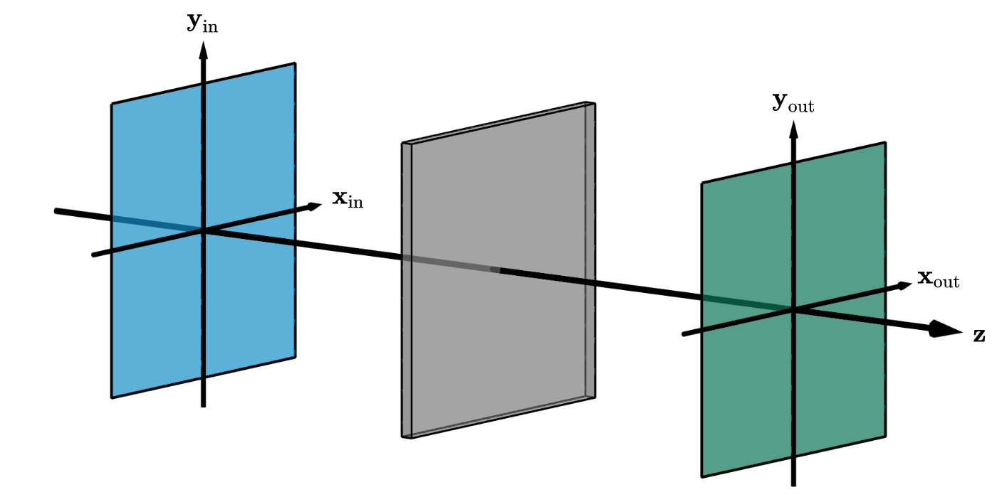
Figure 3: Incident (blue) and outgoing (green) Stokes reference frames in the case with collinear directions.

For the general case, e.g. a Mueller matrix that describes a reflection on some interface, the two frames are necessarily different and need to be tracked carefully:

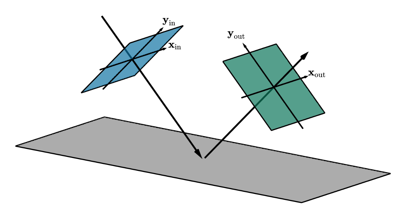
Figure 4: Incident (blue) and outgoing (green) Stokes reference frames in the general case of reflection.

Warning

Stokes and Mueller matrix operations

A lot of care has to be taken when operating with Stokes vectors and Mueller matrices.

1. Matrix multiplication between Mueller matrix and Stokes vector \(\mathbf{s}_{\text{out}} = \mathbf{M} \cdot \mathbf{s}_{\text{in}}\) like above is only valid if the incident reference frame of \(\mathbf{M}\) is equivalent to the reference frame of \(\mathbf{s}_{\text{in}}\).

2. Mueller matrix multiplication \(\mathbf{M}_2 \cdot \mathbf{M}_1\) is only valid if the outgoing frame of \(\mathbf{M}_1\) is aligned with the incident frame of \(\mathbf{M}_2\). Like normal matrix multiplication, this operation does not commute in general.

3. Mueller matrices need to be left multiplied onto Stokes vectors. For instance, \(\mathbf{M}_2 \cdot \mathbf{M}_1 \cdot \mathbf{s}_{\text{in}}\) indicates that a light beam (with Stokes vector \(\mathbf{s}_{\text{in}}\)) first interacts with \(\mathbf{M}_1\) followed by \(\mathbf{M}_2\).

Apart from standard optical elements (Table 2) and other a few other idealized cases, interaction of polarized light with arbitrary materials is not well understood at this point. We will cover the important special case of specular reflection or refraction later in Section Fresnel equations.

Description	Mueller matrix
Ideal depolarizer	\(\begin{bmatrix} 1 & 0 & 0 & 0 \\ 0 & 0 & 0 & 0 \\ 0 & 0 & 0 & 0 \\ 0 & 0 & 0 & 0 \end{bmatrix}\)
Attenuation filter, \(\alpha\): transmission	\(\alpha \begin{bmatrix} 1 & 0 & 0 & 0 \\ 0 & 1 & 0 & 0 \\ 0 & 0 & 1 & 0 \\ 0 & 0 & 0 & 1 \end{bmatrix}\)
Ideal linear polarizer (horizontal transmission)	\(\frac{1}{2} \begin{bmatrix} 1 & 1 & 0 & 0 \\ 1 & 1 & 0 & 0 \\ 0 & 0 & 0 & 0 \\ 0 & 0 & 0 & 0 \end{bmatrix}\)
Ideal linear retarder (fast axis horizontal), \(\phi\): phase difference	\(\begin{bmatrix} 1 & 0 & 0 & 0 \\ 0 & 1 & 0 & 0 \\ 0 & 0 & \cos\phi & \sin\phi \\ 0 & 0 & -\sin\phi & \cos\phi \end{bmatrix}\)
Ideal quarter-wave plate (fast axis horizontal)	\(\begin{bmatrix} 1 & 0 & 0 & 0 \\ 0 & 1 & 0 & 0 \\ 0 & 0 & 0 & 1 \\ 0 & 0 & -1 & 0 \end{bmatrix}\)
Ideal half-wave plate	\(\begin{bmatrix} 1 & 0 & 0 & 0 \\ 0 & 1 & 0 & 0 \\ 0 & 0 & -1 & 0 \\ 0 & 0 & 0 & -1 \end{bmatrix}\)
Ideal right circular polarizer	\(\frac{1}{2} \begin{bmatrix} 1 & 0 & 0 & 1 \\ 0 & 0 & 0 & 0 \\ 0 & 0 & 0 & 0 \\ 1 & 0 & 0 & 1 \end{bmatrix}\)
Ideal left circular polarizer	\(\frac{1}{2} \begin{bmatrix} 1 & 0 & 0 & -1 \\ 0 & 0 & 0 & 0 \\ 0 & 0 & 0 & 0 \\ -1 & 0 & 0 & 1 \end{bmatrix}\)
General polarizer. \(\alpha_x, \alpha_y\): transmission along the two orthogonal axes	\(\frac{1}{2} \begin{bmatrix} \alpha_x^2 + \alpha_y^2 & \alpha_x^2 - \alpha_y^2 & 0 & 0 \\ \alpha_x^2 - \alpha_y^2 & \alpha_x^2 + \alpha_y^2 & 0 & 0 \\ 0 & 0 & 2 \alpha_x \alpha_y & 0 \\ 0 & 0 & 0 & 2 \alpha_x \alpha_y \end{bmatrix}\)

Table 2 A list of Mueller matrices for typical optical elements.

Rotation of Stokes vector frames

Due to the importance of applying Mueller matrices on Stokes vectors only when expressed in the same reference frames, we often have to perform rotations of these frames during a simulation of polarized light. This is somewhat unintuitive at first and can be a source of common errors in an implementation.

We already briefly touched on how rotations of reference frames change how e.g. a Stokes vector is measured (see Figure 2) and we will now formalize the rotation operation as yet another Mueller matrix \(\mathbf{R}(\theta)\) [[4]] that can be applied to a Stokes vector \(\mathbf{s}\) to express it in another reference frame that was rotated by an angle \(\theta\) (measured counter-clockwise from the \(\mathbf{x}\)-axis). This new Stokes vector is then

(2)\[\begin{equation} \mathbf{s}' = \mathbf{R}(\theta) \cdot \mathbf{s} \end{equation}\]

with the rotator matrix defined as

(3)\[\begin{split}\begin{equation} \mathbf{R}(\theta) = \begin{bmatrix} 1 & 0 & 0 & 0 \\ 0 & \cos(2\theta) & \sin(2\theta) & 0 \\ 0 & -\sin(2\theta) & \cos(2\theta) & 0 \\ 0 & 0 & 0 & 1 \end{bmatrix} \end{equation}\end{split}\]

Here is another visualization of this process. Again, note how the polarization of light did not actually change globally, but only expressed relative to the used reference frames:

Rotation of Mueller matrix frames

This idea of rotating the Stokes reference frames can naturally be used to address the challenges of Mueller matrix multiplications involving mismatched frames from above. Consider Figure 5 below.

We want to apply some Mueller matrix \(\hat{\mathbf{M}}\) that operates from reference frame (\(\hat{\mathbf{x}}_{\text{in}}, \hat{\mathbf{y}}_{\text{in}}\)) to (\(\hat{\mathbf{x}}_{\text{out}}, \hat{\mathbf{y}}_{\text{out}}\)) to an incoming beam of light with Stokes vector \(\mathbf{s}\) that is defined relative to the frame (\(\mathbf{x}_{\text{in}}, \mathbf{y}_{\text{in}}\)). As the mismatch makes this impossible, we have to first rotate the incident Stokes vector to be expressed in the different frame:

(4)\[\begin{equation} \mathbf{s}' = \mathbf{R}(\theta_{\text{in}}) \cdot \mathbf{s} \end{equation}\]

where \(\theta_{\text{in}}\) is the relative angle between the two frame bases \(\mathbf{x}_{\text{in}}\) and \(\hat{\mathbf{x}}_{\text{in}}\).

We can then apply the matrix \(\hat{\mathbf{M}}\), as it is valid for the incident frame (\(\hat{\mathbf{x}}_{\text{in}}, \hat{\mathbf{y}}_{\text{in}}\)):

(5)\[\begin{equation} \mathbf{s}'' = \hat{\mathbf{M}} \cdot \mathbf{s}' = \hat{\mathbf{M}} \cdot \mathbf{R}(\theta_{\text{in}}) \cdot \mathbf{s} \end{equation}\]

The resulting Stokes vector \(\mathbf{s}''\) is now valid with respect to the frame (\(\hat{\mathbf{x}}_{\text{out}}, \hat{\mathbf{y}}_{\text{out}}\)). As a last step, we might want to, yet again, rotate its frame to be aligned with some other (arbitrary) reference frame (\(\mathbf{x}_{\text{out}}, \mathbf{y}_{\text{out}}\)):

(6)\[\begin{equation} \mathbf{s}''' = \mathbf{R}(\theta_{\text{out}}) \cdot \mathbf{s}'' = \underbrace{\mathbf{R}(\theta_{\text{out}}) \cdot \hat{\mathbf{M}} \cdot \mathbf{R}(\theta_{\text{in}})}_{\mathbf{M}} \cdot \mathbf{s} \end{equation}\]

where \(\theta_{\text{out}}\) is the relative angle between the two frame bases \(\hat{\mathbf{x}}_{\text{out}}\) and \(\mathbf{x}_{\text{out}}\).

Effectively, this process transforms the matrix \(\hat{\mathbf{M}}\) into a modified matrix \(\mathbf{M}\) that operates between rotated incident and outgoing frames.

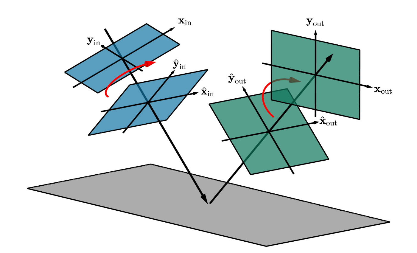
Figure 5: Rotation of Mueller matrix incident and outgoing reference frames.

Rotation of optical elements

Another common use case of the reference frame rotations is to find expressions for rotated optical elements. Consider Figure 6 for the following explanation. The optical element with Mueller matrix \(\mathbf{M}\) (valid for incident & outgoing frame (\(\mathbf{x}', \mathbf{y}'\))) is rotated by an angle \(\theta\). We now want to find the Mueller matrix \(\mathbf{M}(\theta)\) of this rotated element, expressed for incident and outgoing frame (\(\mathbf{x}, \mathbf{y}\)) that is aligned with the optical table. We again achieve this using two rotations, and the steps are analogous to the description above (Section Rotation of Mueller matrix frames):

First we rotate the incident Stokes vector to be expressed in the rotated frame:

(7)\[\begin{equation} \mathbf{s}' = \mathbf{R}(\theta) \cdot \mathbf{s} \end{equation}\]

We then apply the matrix \(\mathbf{M}\), as it is valid for the frame (\(\mathbf{x}', \mathbf{y}'\)):

(8)\[\begin{equation} \mathbf{s}'' = \mathbf{M} \cdot \mathbf{s}' = \mathbf{M} \cdot \mathbf{R}(\theta) \cdot \mathbf{s} \end{equation}\]

Finally, we rotate the resulting Stokes vector back into the original frame (\(\mathbf{x}, \mathbf{y}\)):

(9)\[\begin{equation} \mathbf{s}''' = \mathbf{R}(-\theta) \cdot \mathbf{s}'' = \underbrace{\mathbf{R}(-\theta) \cdot \mathbf{M} \cdot \mathbf{R}(\theta)}_{\mathbf{M}(\theta)} \cdot \mathbf{s} \end{equation}\]

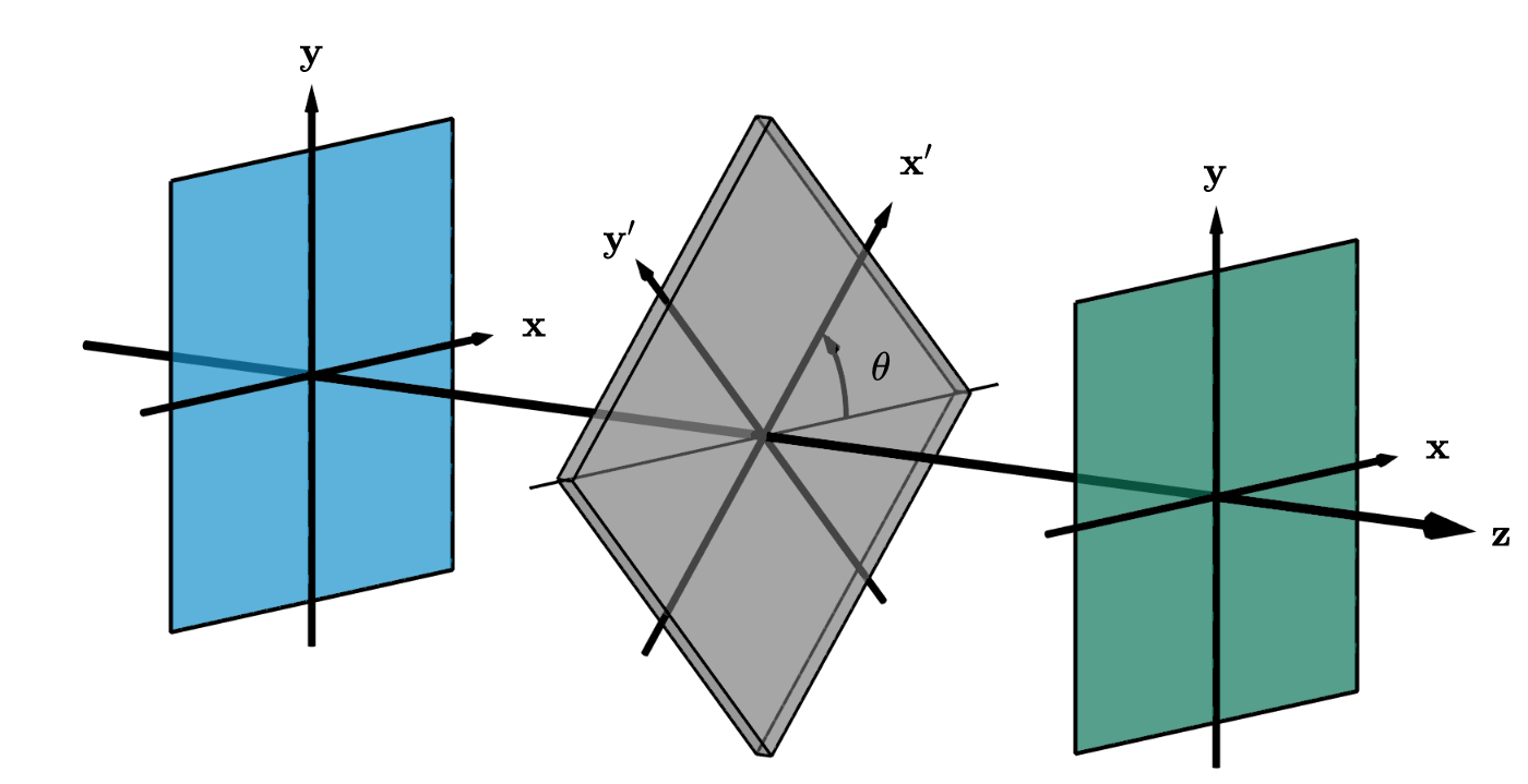
Figure 6: An optical element rotated around the axis of propagation.

Example 1: A rotated linear polarizer

A very common special case of this is a linear polarizer rotated at some angle. Recall the Mueller matrix of a linear polarizer:

(10)\[\begin{split}\begin{equation} \mathbf{L} = \frac{1}{2} \begin{bmatrix} 1 & 1 & 0 & 0 \\ 1 & 1 & 0 & 0 \\ 0 & 0 & 0 & 0 \\ 0 & 0 & 0 & 0 \end{bmatrix} \end{equation}\end{split}\]

When applying Eq. (9) to Eq. (10) we get the expression

(11)\[\begin{split}\begin{equation} \mathbf{L}(\theta) = \frac{1}{2} \begin{bmatrix} 1 & \cos(2\theta) & \sin(2\theta) & 0 \\ \cos(2\theta) & \cos^2(2\theta) & \sin(2\theta)\cos(2\theta) & 0 \\ \sin(2\theta) & \sin(2\theta)\cos(2\theta) & \sin^2(2\theta) & 0 \\ 0 & 0 & 0 & 0 \end{bmatrix} \end{equation}.\end{split}\]

Example 2: Malus’ law

Consider a beam of unpolarized light (purple) that interacts with two linear polarizers as illustrated here:

The first polarizer transforms the beam into fully horizontally polarized light (middle) before traveling through a second polarizer at an angle \(\theta\). It is clear that a horizontal orientation (\(\theta=0˚\)) will allow all of the light to transmit as both polarizers are aligned with each other. Similarly, at an orthogonal configuration (\(\theta=90˚\)), all light will be absorbed. For intermediate angles, only a fraction of the light is transmitted in form of linearly polarized light. Under such a setting, the total intensities (first component of the Stokes vector) before and after interacting with the two polarizers, \(\mathbf{s}_0, \mathbf{s}_0'\), follow Malus’ law [[5]]:

(12)\[\begin{equation} \mathbf{s}_0' = \frac{\cos^2(\theta)}{2} \cdot \mathbf{s}_0 \end{equation}\]

where \(\theta\) is the rotation angle of the second polarizer, measured counter-clockwise from the horizontal configuration.

This can easily be derived by in the Mueller-Stokes calculus, simply by left multiplying the matrices in Eq. (10) and Eq. (11) onto some arbitrary Stokes vector \(\mathbf{s}\):

\[\begin{split}\begin{align*} \begin{bmatrix} \mathbf{s}_0' \\ \mathbf{s}_1' \\ \mathbf{s}_2' \\ \mathbf{s}_3' \end{bmatrix} &= \mathbf{L}(\theta) \cdot \mathbf{L} \cdot \begin{bmatrix} \mathbf{s}_0 \\ \mathbf{s}_1 \\ \mathbf{s}_2 \\ \mathbf{s}_3 \end{bmatrix} \\ &= \frac{1}{4} \begin{bmatrix} 1 & \cos(2\theta) & \sin(2\theta) & 0 \\ \cos(2\theta) & \cos^{2}(2\theta) & \sin(2\theta)\cos(2\theta) & 0 \\ \sin(2\theta) & \sin(2\theta)\cos(2\theta) & \sin^{2}(2\theta) & 0 \\ 0 & 0 & 0 & 0 \end{bmatrix} \cdot \begin{bmatrix} 1 & 1 & 0 & 0 \\ 1 & 1 & 0 & 0 \\ 0 & 0 & 0 & 0 \\ 0 & 0 & 0 & 0 \end{bmatrix} \cdot \begin{bmatrix} \mathbf{s}_0 \\ \mathbf{s}_1 \\ \mathbf{s}_2 \\ \mathbf{s}_3 \end{bmatrix} \\ &= \frac{1}{4} \begin{bmatrix} 1 & \cos(2\theta) & \sin(2\theta) & 0 \\ \cos(2\theta) & \cos^{2}(2\theta) & \sin(2\theta)\cos(2\theta) & 0 \\ \sin(2\theta) & \sin(2\theta)\cos(2\theta) & \sin^{2}(2\theta) & 0 \\ 0 & 0 & 0 & 0 \end{bmatrix} \cdot \begin{bmatrix} \mathbf{s}_0 + \mathbf{s}_1 \\ \mathbf{s}_0 + \mathbf{s}_1 \\ 0 \\ 0 \end{bmatrix} \\ &= \frac{1}{4} \begin{bmatrix} (\mathbf{s}_0 + \mathbf{s}_1) (1 + \cos(2\theta)) \\ (\mathbf{s}_0 + \mathbf{s}_1) (1 + \cos(2\theta))\cos(2\theta) \\ (\mathbf{s}_0 + \mathbf{s}_1) (1 + \cos(2\theta))\sin(2\theta) \\ 0 \end{bmatrix} \\ &= \frac{1}{2} \begin{bmatrix} (\mathbf{s}_0 + \mathbf{s}_1) (\cos^{2}\theta) \\ (\mathbf{s}_0 + \mathbf{s}_1) (\cos^{2}\theta)\cos(2\theta) \\ (\mathbf{s}_0 + \mathbf{s}_1) (\cos^{2}\theta)\sin(2\theta) \\ 0 \end{bmatrix} \end{align*}\end{split}\]

Here, the last step used the trigonometric identity \(\cos(2\theta) = 2\cos^{2}\theta - 1\). Plugging in the Stokes vector of unpolarized light (\(\mathbf{s}_0 = 1, \mathbf{s}_1=\mathbf{s}_2=\mathbf{s}_3=0\)) directly gives Eq. (12) as result.

Example 3: Creation of circular polarization

We can also use Mueller-Stokes calculus to understand a common physical setup to create circularly polarized light that uses a clever combination of a linear polarizer and a quarter-wave plate:

Any type of light (e.g. unpolarized, visualized in purple) is linearly polarized at a 45˚ angle by the first filter (left) and then hits a quarter-wave plate (green) that has its “fast axis” in a horizontal configuration. The wave plate introduces a quarter wavelength phase shift that slows down the vertical component (red). As a result, the two wave components are no longer aligned and the light beam is (perfectly) left-circularly polarized.

Or written in Mueller-Stokes calculus, using the quarter-wave plate from Table 2 and the rotated linear polarizer from Eq. (11) using \(\theta=45˚\):

\[\begin{split}\begin{align*} \begin{bmatrix} \mathbf{s}_0' \\ \mathbf{s}_1' \\ \mathbf{s}_2' \\ \mathbf{s}_3' \end{bmatrix} &= \frac{1}{2} \begin{bmatrix} 1 & 0 & 0 & 0 \\ 0 & 1 & 0 & 0 \\ 0 & 0 & 0 & 1 \\ 0 & 0 & -1 & 0 \end{bmatrix} \cdot \begin{bmatrix} 1 & \cos(2\theta) & \sin(2\theta) & 0 \\ \cos(2\theta) & \cos^{2}(2\theta) & \sin(2\theta)\cos(2\theta) & 0 \\ \sin(2\theta) & \sin(2\theta)\cos(2\theta) & \sin^{2}(2\theta) & 0 \\ 0 & 0 & 0 & 0 \end{bmatrix} \cdot \begin{bmatrix} \mathbf{s}_0 \\ \mathbf{s}_1 \\ \mathbf{s}_2 \\ \mathbf{s}_3 \end{bmatrix} \\ &= \frac{1}{2} \begin{bmatrix} 1 & 0 & 0 & 0 \\ 0 & 1 & 0 & 0 \\ 0 & 0 & 0 & 1 \\ 0 & 0 & -1 & 0 \end{bmatrix} \cdot \begin{bmatrix} \mathbf{s}_0 + \mathbf{s}_2 \\ 0 \\ \mathbf{s}_0 + \mathbf{s}_2 \\ 0 \end{bmatrix} \\ &= \frac{1}{2} \begin{bmatrix} \mathbf{s}_0 + \mathbf{s}_2 \\ 0 \\ 0 \\ -(\mathbf{s}_0 + \mathbf{s}_2) \end{bmatrix} \end{align*}\end{split}\]

To figure out the signs of the final Stokes vector, recall that \(\mathbf{s}_0 \geq \sqrt{\mathbf{s}_1^2 + \mathbf{s}_2^2 + \mathbf{s}_3^2}\). From this we have \((\mathbf{s}_0 + \mathbf{s}_2) > 0\) and thus the last entry has to be negative which matches the observed left-circular polarization above.

---

[4]

Note that this Mueller matrix of a rotator does not correspond to an actual optical element one could use in a practical setup. It is only used to reason about how the Stokes vector expression changes when viewed from a differently oriented reference frame.

[5]

The factor \(\frac{1}{2}\) comes from the fact that we start out with unpolarized light. Many sources omit this factor but instead relate intensity before and after the second (rotated) polarizer.

Fresnel equations

Specular dielectrics and conductors are important building blocks of material models in most rendering systems today. They are usually based on the well known Fresnel equations (first derived by Augustin Jean Fresnel in the 19th century [Fre23]) that describe the complete polarization state of specular reflection and refraction on such materials. Note that this is one of the few cases where exact expressions are available and therefore we definitely want to accurately capture this effect in polarization aware rendering.

At the core of this are of course the laws of reflection and refraction (a.k.a. Snell’s law)

(13)\[\begin{split}\begin{align} \textbf{Reflection}: \;\;& \theta_i = \theta_r \\ \textbf{Refraction}: \;\;& \eta_i \cdot \sin\theta_i = \eta_t \cdot \sin\theta_t \end{align}\end{split}\]

that relate an incident angle \(\theta_i\) with its reflected (\(\theta_r\)) and refracted (\(\theta_t\)) analogues based on the indices of refraction (\(\eta_i \text{ and } \eta_t\)) on the two sides of the interface:

A typical example would be light that refracts from air into a denser medium such as water. In this case, we have \(\eta_i \approx 1.0\) and \(\eta_t \approx 1.33\).

Theory

Modern formulations of the Fresnel equations are based on electromagnetic theory [[6]] where we consider the two transverse fields \(E\) (electric) and \(H\) (magnetic). Usually, derivations relate the incident (\(E_i\)) with the reflected (\(E_r\)) and transmitted (\(E_t\)) electric fields, though equivalently the magnetic fields could also be used. It is sufficient to consider two cases where the electric field arrives either in perpendicular (”\(\bot\)”) or parallel (”\(\parallel\)”) orientation relative to the plane of incidence [[7]]:

To describe these fields, we have to make some choices regarding coordinate systems. In particular: in which directions should the electric fields be pointing before and after interacting with the interface? Given the electric field direction \(E\) and the propagation direction of the beam \(\mathbf{z}\), the orientation of the magnetic field \(H\) is always clearly defined by a right-handed coordinate system \(E \times H = \alpha \cdot \mathbf{z}\) for some constant \(\alpha\) (Poynting’s theorem). The orientation of the electric field itself is however somewhat arbitrary. Incident and reflected field could for instance point in the same or opposite directions of each other.

Warning

Electric field conventions

Unfortunately, different choices for the orientations of the electric field will result in slightly different versions of the final Fresnel equations. All versions are “correct” however as long as conventions are clear and consistent. We therefore clarify the concrete alignments that we use in the following diagram:

Figure 7: The convention we use for directions of the electric (\(E\)) and magnetic (\(H\)) fields in case of specular reflection and transmission. In this configuration, all electric fields are parallel to each other which also known as the Verdet convention in the literature.

Perpendicular electric field

In this case (Figure 7 (a)) all electric field vectors \(E_i^{\bot}, E_r^{\bot}\), and \(E_t^{\bot}\) are collinear. It is therefore the most natural to orient them all in the same direction, e.g. pointing into the screen / plane. In fact, practically all sources agree on this convention [Muller69].

Parallel electric field

Here, the three vectors \(E_i^{\bot}, E_r^{\bot}\), and \(E_t^{\bot}\) are coplanar but (for general \(\theta_i\)) not collinear anymore and it is therefore not so clear what it means to “point into the same direction”. Instead, this is now defined based on the magnetic field vectors \(H_i^{\bot}, H_r^{\bot}\), and \(H_t^{\bot}\) which are collinear.

In Figure 7 (b), we decided to have them all point into the same direction again which is commonly referred to as the Verdet convention in the literature. Most sources agree on the directions of \(E_i^{\parallel}\) vs. \(E_t^{\parallel}\) in the transmission case. However a large number of them choose to orient \(E_r^{\parallel}\) (and \(H_r^{\parallel}\)) in the opposite direction [Muller69], also known as the Fresnel convention. Such a sign flip will propagate all the way into the signs of the Fresnel equations but it is important to keep in mind that both are “correct” based on the chosen coordinate systems. See Section Different conventions in the literature below for an extended discussion.

Equations

Based on the chosen convention above, we now summarize the Fresnel equations as implemented in Mitsuba 3. For the purpose of this document we omit their actual derivations and instead refer interested readers to Optics by E. Hecht [Hec98].

The reflection amplitude coefficients for the “\(\bot\)” and “\(\parallel\)” components relate the incident and reflected electric fields via

(14)\[\begin{align} r_{\bot} = \frac{E_r^{\bot}}{E_i^{\bot}} = \frac{\eta_i \cos\theta_i - \eta_t \cos\theta_t}{\eta_i \cos\theta_i + \eta_t \cos\theta_t} = -\frac{\sin(\theta_i - \theta_t)}{\sin(\theta_i + \theta_t)} \end{align}\]

(15)\[\begin{align} r_{\parallel} = \frac{E_r^{\parallel}}{E_i^{\parallel}} = \frac{\eta_t \cos\theta_i - \eta_i \cos\theta_t}{\eta_t \cos\theta_i + \eta_i \cos\theta_t} = +\frac{\tan(\theta_i - \theta_t)}{\tan(\theta_i + \theta_t)} \end{align}\]

where \(\cos\theta_t\) can be computed from Snell’s law (Eq. (13)) as \(\cos\theta_t = \sqrt{1 - {\left(\frac{\eta_i}{\eta_t}\right)}^{2} {\sin}^{2}\theta_i}\). A negative value under the square root in this expression usually indicates that refraction is impossible, and instead all light is reflected (the total internal reflection case) but here, the complex valued square root is used as part of Eq. (14) and Eq. (15).

Note that the leading signs of both equations would change based on different conventions for the electric field orientations above.

The same expressions also hold in the conductor case where the indices of refraction are complex valued, i.e. \(\eta = n - k i\) with real and imaginary parts \(n\) and \(k\). The use of complex numbers here comes from the expression \(\exp(-i \, \alpha \, \eta \, t)\) that describes a plane wave propagating with increasing time \(t\) and a constant \(\alpha\) related to the wave frequency. When introducing a value of \(k > 0\), this now leads to an exponential decay of the wave as it travels inside the conductor material: \(\exp(-i \, n \, \alpha \, t) \cdot \exp(-\alpha \, k \, t)\). For that reason, \(k\) is also known as the extinction coefficient.

There exist alternate conventions of this description where the direction of the time dependence is reversed (\(\exp(+i \, \alpha \, \eta \, t)\)) and as a consequence, the sign of the complex component is flipped to (\(n + k i\)) [Muller69]. We use the former convention with the negative sign (\(n - k i\)) in this document.

---

Similarly, we can use the complex amplitudes after refraction to determine the transmission amplitude coefficients, where a few different expressions are commonly found:

(16)\[\begin{align} t_{\bot} &= \frac{E_t^{\bot}}{E_i^{\bot}} = \frac{2 \cos\theta_i \sin\theta_t}{\sin(\theta_i + \theta_t)} = \frac{2 \eta_i \cos\theta_i}{\eta_i \cos\theta_i + \eta_t \cos\theta_t} \end{align}\]

(17)\[\begin{align} t_{\parallel} &= \frac{E_t^{\parallel}}{E_i^{\parallel}} = \frac{2 \cos\theta_i \sin\theta_t}{\sin(\theta_i + \theta_t) \cos(\theta_i - \theta_t)} = \frac{2 \eta_i \cos\theta_i}{\eta_t \cos\theta_i + \eta_i \cos\theta_t} \end{align}\]

where, as mentioned above, most sources seem to agree on the signs. A particular simple expression of these is also available in case the reflection coefficients have already been computed:

(18)\[\begin{align} t_{\bot} = 1 + r_{\bot}, \;\;\;\;\; t_{\parallel} = (1 + r_{\parallel}) \frac{\eta_i}{\eta_t} \end{align}\]

Obviously, these last expression now depend on the choice of the electric field directions again.

---

The complex reflection amplitudes also encode the phase shifts of the respective wave components. The relative phase shift between “\(\parallel\)” and “\(\bot\)” components is given by

(19)\[\begin{align} \Delta = \delta_\parallel - \delta_\bot = \arg(r_\parallel) - \arg(r_\bot) \end{align}\]

where both \(\delta_\parallel\) and \(\delta_\bot\) (when positive valued) are phase advances when time is measured to increase in the positive direction [Muller69].

The transmission amplitudes \(t_\bot\) and \(t_\parallel\) are always real valued and refraction therefore does not cause any phase shifts.

---

Two more important quantities are the reflectance (R) and transmittance (T):

(20)\[\begin{align} R = \frac{\text{reflected power}}{\text{incident power}} = \frac{A_r I_r}{A_i I_i} \end{align}\]

(21)\[\begin{align} T = \frac{\text{transmitted power}}{\text{incident power}} = \frac{A_t I_t}{A_i I_i} \end{align}\]

where \(A\) is the beam’s area and \(I\) is the intensity

(22)\[\begin{align} I = \eta \frac{c_0 \, \epsilon_0}{2} {|E|}^{2} \end{align}\]

with refractive index \(\eta\), speed of light (in vacuum) \(c_0\), vacuum permittivity \(\epsilon_0\), and electric field \(E\).

The beam area ratios are found by simple trigonometry to be \(\frac{A_r}{A_i} = \frac{\cos\theta_i}{\cos\theta_i} = 1\) and \(\frac{A_t}{A_i} = \frac{\cos\theta_t}{\cos\theta_i}\):

from which we have the final expressions

(23)\[\begin{align} R = \frac{\eta_i {|E_r|}^{2}}{\eta_i {|E_i|}^{2}} = |r|^{2} \end{align}\]

(24)\[\begin{align} T = \frac{\cos\theta_t \eta_t {|E_t|}^{2}}{\cos\theta_i \eta_i {|E_i|}^{2}} = \frac{\cos\theta_t}{\cos\theta_i } \frac{\eta_t}{\eta_i} |t|^{2} \end{align}\]

From energy conservation, we always have \(R_{\bot} + T_{\bot} = 1\) and \(R_{\parallel} + T_{\parallel}\) = 1, even though the same does not always hold for the amplitudes \(r\) and \(t\).

Different conventions in the literature

When considering all possible orientations of the electric field vectors (2 choices for \(E_i\), \(E_r\), and \(E_t\) for both “\(\bot\)” and “\(\parallel\)”) there seem to 16 different versions. Luckily, many of them are equivalent and from the few remaining ones, the literature is mostly divided into two groups which orient the reflected electric field vector \(E_r^{\parallel}\) differently:

1. Fresnel convention

Here, \(E_i^{\parallel}\) and \(E_r^{\parallel}\) are oriented s.t. their magnetic fields \(H_i^{\bot}\) and \(H_r^{\bot}\) point in opposite directions (Figure 8 below). Its name comes from the fact that it is close to Fresnel’s original description of the equations where both perpendicular and parallel amplitudes (Eq. (14) and Eq. (15)) would use the same sign.

Its main appeal is that at perpendicular incidence, both \(E_i^{\parallel}\) and \(E_r^{\parallel}\) are indistinguishable which makes sense from a physical perspective. However, it accomplishes this by having \(E_r^{\bot}\) & \(E_r^{\parallel}\) form a left handed coordinate system which can be less convenient for subsequent calculations.

Figure 8: The Fresnel convention is a common alternative of orienting the electric fields. The difference to the Verdet convention is a change of handedness of the \(H_r^{\bot}\) and \(E_r^{\parallel}\) frame of the reflected direction highlighted in red.

2. Verdet convention

Here, \(E_i^{\parallel}\) and \(E_r^{\parallel}\) are oriented s.t. their magnetic fields \(H_i^{\bot}\) and \(H_r^{\bot}\) point in the same direction (Figure 7 and repeated below as Figure 9 for easier comparison). It is named after Verdet, who was an editor of Fresnel and originally switched the convention because in his opinion, the two fields should instead be equivalent at grazing angles [PP97], [Cla09]. Compared to Fresnel’s original formulation of the equations, the sign of the parallel amplitude consequently had to be flipped, see Eq. (15).

Figure 9: The convention we use for directions of the electric (\(E\)) and magnetic (\(H\)) fields in case of specular reflection and transmission. In this configuration, all electric fields are parallel to each other which also known as the Verdet convention in the literature.

Because the conventions involve changing the coordinate system orientations, the sign change between the resulting variants of the Fresnel equations can also just be interpreted as phase shift of \(180˚\). However we should emphasize again that, despite their different formulations, all conventions are ultimately correct in their frame of reference — as long as they are clearly defined and used consistently.

---

Apart from these different coordinate systems, and the few other conventions we mentioned before (e.g. time dependence of the waves vs. the complex index of refraction in Section Equations) there are also numerous other aspects of polarization that are not universally agreed upon. We found the the 1969 paper by Muller [Muller69] very useful to understand the space of possibilities and we adopt all conventions recommended in that article. (More precisely the final variants suggested by H. E. Bennett in the discussion section at the end.) Other useful resource to us were [Hec98], [PP97], [BDE+09], [HS80], [FS65], [OV20], [Salik12], [Azz04].

Ultimately, each convention has its own justifications and use cases in different branches of science and a lack of consistency is thus understandable. Nonetheless it is an unfortunate circumstance, especially for anyone new to the theory of polarization.

---

[6]

It is remarkable that the original derivation by Fresnel predates Maxwell’s work on electromagnetic theory and only relied on the elastic-solid theory.

[7]

The literature often also uses letters “S” and “P” for perpendicular and parallel oscillations based on the German words “senkrecht” and “parallel”.

Analysis and Mueller matrix formulation

We now turn to discussing the Fresnel equations in the various cases of reflection and transmission for dielectrics and conductors. At the same time, we will state the corresponding Mueller matrices that encode the laws as part of the Mueller-Stokes calculus used in the renderer. This conversion (when following all conventions from above) is straightforward and was first discussed by Collett [Col71]. At the end, in Section Different conventions in the context of Mueller matrices we will briefly return to some of the alternative conventions and how they sometimes affect Mueller matrix definitions in the literature.

Dielectric reflection (at a denser medium)

The first case is simple dielectric reflection at an interface that is denser than the incident medium. Consider for instance Figure 10 with \(\eta_i = 1.0\) and \(\eta_t = 1.5\). The curves with “\(\bot\)” and “\(\parallel\)” components of the reflectance is also well known in graphics where usually rendering systems implement the non-polarized version \(R_{avg} = R_\bot + R_\parallel\) that just averages the two curves.

Figure 10: Reflectance, phase shifts, and degree of polarization (DOP) for varying incident angle of a specular reflection at the outside of a dielectric interface with relative IOR of \(3/2\) (\(\eta_i = 1.0, \eta_t = 1.5\)).

The angle \(\theta = \arctan(\eta_t / \eta_i)\), also known as Brewster’s angle is of special importance here, as it has several interesting properties:

1. The “\(\parallel\)” reflectance is zero.

2. A phase shift of \(180˚\) takes place which is comparable to a half-wave plate. Note that such a discontinuous “jump” might at first seem implausible but the underlying physics is still continuous because of \(R_\parallel\) smoothly approaching zero at the same time.

3. The light is fully polarized and oscillates along the “\(\bot\)” component (horizontally with respect to the reference frame (\(\mathbf{x}, \mathbf{y}\))).

The Mueller matrix for this case follows the shape of a standard polarizer (see Table 2) where we know how much energy is preserved at the two orthogonal components “\(\bot\)” (horizontal) and “\(\parallel\)” (vertical):

(25)\[\begin{split}\begin{equation} \frac{1}{2} \cdot \begin{bmatrix} R_{\bot} + R_{\parallel} & R_{\bot} - R_{\parallel} & 0 & 0 \\ R_{\bot} - R_{\parallel} & R_{\bot} + R_{\parallel} & 0 & 0 \\ 0 & 0 & 2 \sqrt{R_{\bot} R_{\parallel}} & 0 \\ 0 & 0 & 0 & 2 \sqrt{R_{\bot} R_{\parallel}} \end{bmatrix} \end{equation}\end{split}\]

Dielectric transmission (into a denser medium)

An analogous case is refraction into a medium of higher density as shown in Figure 11 for \(\eta_i = 1.0\) and \(\eta_t = 1.5\).

Figure 11: Transmittance and phase shifts for varying incident angles of a specular refraction from vacuum (\(\eta_i = 1.0\)) into a dielectric (\(\eta_t = 1.5\)).

As discusses previously, there is no phase shift for transmission (the transmission amplitude coefficients are always real). The matrix is also analogous to above:

(26)\[\begin{split}\begin{equation} \frac{1}{2} \cdot \begin{bmatrix} T_{\bot} + T_{\parallel} & T_{\bot} - T_{\parallel} & 0 & 0 \\ T_{\bot} - T_{\parallel} & T_{\bot} + T_{\parallel} & 0 & 0 \\ 0 & 0 & 2 \sqrt{T_{\bot} T_{\parallel}} & 0 \\ 0 & 0 & 0 & 2 \sqrt{T_{\bot} T_{\parallel}} \end{bmatrix} \end{equation}\end{split}\]

Dielectric reflection and transmission (from a denser to a less dense medium)

Internal reflection inside a dense dielectric (\(\eta_t / \eta_i < 1\)) is an interesting case due to the well known critical angle (\(\theta = \arcsin(\eta_t / \eta_i)\)) after which all light is reflected and thus transmittance goes to zero. This is also known as total internal reflection (TIR) See e.g. Figure 12 for the reflection case and Figure 13 for transmission in case of \(\eta_i = 1.5\) and \(\eta_t = 1.0\).

Figure 12: Reflectance and phase shifts for varying incident angles of a specular reflection from the inside of a dielectric interface with relative IOR \(2/3\) (\(\eta_i = 1.5, \eta_t = 1.0\)). Compare also with Fig. 1 in [Azz04].

Figure 13: Transmittance and phase shifts for varying incident angles of a specular refraction from a dielectric (\(\eta_i = 1.0\)) into vacuum (\(\eta_t = 1.5\)).

The phase shifts in this case were studied in detail by Azzam [Azz04]. Similar to the previous case in Section Dielectric reflection (at a denser medium), there is a phase change of \(180˚\) after \(\theta = \arctan(\eta_t / \eta_i)\) but now there is an additional variation in the phase shift for incident directions below the critical angle. It’s maximal value is located at angle

(27)\[\begin{equation} \arg \max_\theta \Delta(\theta) = \arccos\sqrt{\frac{1 - (\eta_t / \eta_i)^2}{1 + (\eta_t / \eta_i)^2}} \end{equation}\]

Because all light is reflected (\(R_\bot = R_\parallel = 1\)) and \(\Delta \neq 0\), the Mueller matrix for the total internal reflection case is just a retarder:

(28)\[\begin{split}\begin{equation} \begin{bmatrix} 1 & 0 & 0 & 0 \\ 0 & 1 & 0 & 0 \\ 0 & 0 & \cos\Delta & -\sin\Delta \\ 0 & 0 & \sin\Delta & \cos\Delta \end{bmatrix} \end{equation}\end{split}\]

The sign is flipped compared to the retarder matrix in Table 2 which is a consequence of using the relative phase shift definition from [Muller69] (Eq. (19)). See Section Different conventions in the context of Mueller matrices for formulations under alternative conventions.

Example: Fresnel rhomb

Fresnel [Fre23] realized that the phase shifts due to total internal reflection can be used to turn linear into circular polarization by constructing a prism where light is is reflected twice on the interior of a dielectric material. The angle have to be chosen carefully based on the refractive index s.t. the correct phase shift of \(90˚\) (i.e. equivalent to a quarter-wave plate) is achieved:

Note that, as seen in Figure 12, a single reflection is not sufficient for typical glass-like materials as the retardation is actually \(< 90˚\). Instead, the two reflections will each cause a shift of \(45˚\). More precisely, the “\(\parallel\)” component will be advanced by \(90˚\) relative to “\(\bot\)”.

A specific example would be \(\eta_i \approx 1.49661\) where the correct shift (\(\Delta = 45˚\)) is achieved with \(\theta_i = \arg \min_\theta \Delta(\theta) \approx 51.782˚\) (Eq. (27)).

Multiplying the Mueller matrices of the two reflections gives

\[\begin{split}\begin{align} \mathbf{M}_{rhomb} &= \begin{bmatrix} 1 & 0 & 0 & 0 \\ 0 & 1 & 0 & 0 \\ 0 & 0 & \cos\Delta & -\sin\Delta \\ 0 & 0 & \sin\Delta & \cos\Delta \end{bmatrix} \cdot \begin{bmatrix} 1 & 0 & 0 & 0 \\ 0 & 1 & 0 & 0 \\ 0 & 0 & \cos\Delta & -\sin\Delta \\ 0 & 0 & \sin\Delta & \cos\Delta \end{bmatrix} \\ &= \begin{bmatrix} 1 & 0 & 0 & 0 \\ 0 & 1 & 0 & 0 \\ 0 & 0 & \cos^{2}\Delta - \sin^{2}\Delta & -2\cos\Delta\sin\Delta \\ 0 & 0 & 2\cos\Delta\sin\Delta & \cos^{2}\Delta - \sin^{2}\Delta \end{bmatrix} = \begin{bmatrix} 1 & 0 & 0 & 0 \\ 0 & 1 & 0 & 0 \\ 0 & 0 & \cos(2\Delta) & -\sin(2\Delta) \\ 0 & 0 & \sin(2\Delta) & \cos(2\Delta) \end{bmatrix} \\ &= \begin{bmatrix} 1 & 0 & 0 & 0 \\ 0 & 1 & 0 & 0 \\ 0 & 0 & 0 & -1 \\ 0 & 0 & 1 & 0 \end{bmatrix} \end{align}\end{split}\]

which is equivalent to a Mueller matrix of a quarter-wave plate with its fast axis vertical, i.e. aligned with “\(\parallel\)”, see Table 2.

Finally, when sending linearly (diagonal at \(+45˚\)) polarized light through the prism, the outgoing light will be right-circularly polarized:

\[\begin{split}\begin{align} \mathbf{M}_{rhomb} \cdot \begin{bmatrix} 1 \\ 0 \\ 1 \\ 0 \end{bmatrix} = \begin{bmatrix} 1 \\ 0 \\ 0 \\ 1 \end{bmatrix} \end{align}\end{split}\]

Conductor reflection

As mentioned at the beginning of Section Theory, all equations also generalize the the case of reflection on conductors that have complex valued indices of refraction \(\eta = n - k i\) where \(n\) is the real part and \(k\) is the extinction coefficient. Figure 14 shows a typical case with \(\eta = 0.183 - 3.43i\) (gold at 633nm).

Figure 14: Reflectance and phase shifts for varying incident angles of a specular reflection on a conductor with complex IOR of \(\eta = 0.183 - 3.43i\). Compare also with Fig. B in [Muller69].

Plugging in complex IORs with the wrong sign convention into the equations here will result in a sign flip between the two \(\sin(...)\) expressions in the matrix below. To avoid any issues in our implementation, Mitsuba 3 will automatically flip the sign appropriately so both conventions of input parameters can be used.

Compared to the dielectric cases earlier, every incident angle results in some phase shift now, and thus the Mueller matrix is a combination of a polarizer and retarder:

(29)\[\begin{split}\begin{equation} \frac{1}{2} \begin{bmatrix} R_{\bot} + R_{\parallel} & R_{\bot} - R_{\parallel} & 0 & 0 \\ R_{\bot} - R_{\parallel} & R_{\bot} + R_{\parallel} & 0 & 0 \\ 0 & 0 & 2 \sqrt{R_{\bot} R_{\parallel}} \cos\Delta & -2 \sqrt{R_{\bot} R_{\parallel}} \sin\Delta \\ 0 & 0 & 2 \sqrt{R_{\bot} R_{\parallel}} \sin\Delta & 2 \sqrt{R_{\bot} R_{\parallel}} \cos\Delta \end{bmatrix} \end{equation}\end{split}\]

The dashed line in Figure 14 also illustrates the principle angle of incidence which is \(\theta_i\) where the relative phase shift is exactly a quarter wavelength (\(90˚\)). It can be used to measure the complex IOR of a metallic material [Col05].

Fully general case (dielectric + conductor) covering all cases

Finally, we can summarize all cases using just two different Mueller matrices for reflection and transmission respectively which makes an implementation less error-prone:

(30)\[\begin{split}\begin{equation} \mathbf{F}_r = \frac{1}{2} \cdot \begin{bmatrix} R_{\bot} + R_{\parallel} & R_{\bot} - R_{\parallel} & 0 & 0 \\ R_{\bot} - R_{\parallel} & R_{\bot} + R_{\parallel} & 0 & 0 \\ 0 & 0 & 2 \sqrt{R_{\bot} R_{\parallel}} \cos\Delta & -2 \sqrt{R_{\bot} R_{\parallel}} \sin\Delta \\ 0 & 0 & 2 \sqrt{R_{\bot} R_{\parallel}} \sin\Delta & 2 \sqrt{R_{\bot} R_{\parallel}} \cos\Delta \end{bmatrix} \end{equation}\end{split}\]

(31)\[\begin{split}\begin{equation} \mathbf{F}_t = \frac{1}{2} \cdot \begin{bmatrix} T_{\bot} + T_{\parallel} & T_{\bot} - T_{\parallel} & 0 & 0 \\ T_{\bot} - T_{\parallel} & T_{\bot} + T_{\parallel} & 0 & 0 \\ 0 & 0 & 2 \sqrt{T_{\bot} T_{\parallel}} & 0 \\ 0 & 0 & 0 & 2 \sqrt{T_{\bot} T_{\parallel}} \end{bmatrix} \end{equation}\end{split}\]

It can be seen how Eq. (30) simplifies back to the simpler case earlier (Eq. (25)) in case the index of refraction is real (dielectric) and no total internal reflection occurs. In that case, the relative phase shift \(\Delta = 0\), so \(\cos\Delta = 1\) and \(\sin\Delta = 0\).

Different conventions in the context of Mueller matrices

Some of the conventions used in other sources of course also affect the Mueller matrix formulations. As a result, the matrices written above exist in the literature in various versions that differ in the signs of the individual entries.

1. Fresnel vs. Verdet convention

In the Fresnel convention (Section Different conventions in the literature), the reflected field vectors \(E_r^{\bot}\) and \(E_r^{\parallel}\) define a left handed coordinate system with the direction of propagation which is incompatible with the usual definitions of the Stokes parameters. As a workaround, in case this convention is used for the Fresnel equations, an additional handedness change matrix

(32)\[\begin{split}\begin{equation} \begin{bmatrix} 1 & 0 & 0 & 0 \\ 0 & 1 & 0 & 0 \\ 0 & 0 & -1 & 0 \\ 0 & 0 & 0 & -1 \end{bmatrix} \end{equation}\end{split}\]

needs to be introduced [Cla09]. Effectively, this is nothing different than the Mueller matrix of a half-wave plate (Table 2) that introduces a \(180˚\) phase shift that switches all signs to the Verdet convention.

This would affect all matrices involving reflections (Eq. (25), Eq. (28), Eq. (29), and Eq. (30)) above.

2. Phase shift definitions

The relative phase shift \(\Delta = \delta_\parallel - \delta_\bot\) between “\(\parallel\)” and “\(\bot\)” (Eq. (19)) is often also presented in opposite form as

(33)\[\begin{align} \Delta' = \delta_\bot - \delta_\parallel = -\Delta \end{align}\]

which will swap the signs of the two \(\sin(\dots)\) expressions in Eq. (28), Eq. (29), and Eq. (30).

3. Phase shift directions

The phase shifts \(\delta_\parallel\) and \(\delta_\bot\) are sometimes also interpreted as phase retardations instead of advances, which also influences the same signs, canceling the previous sign convention (Fresnel vs. Verdet convention) again.

Validation against measurements

Due to the many possible sources of subtle errors and sign flips in the implementation of the Fresnel equation we also validated the output of Mitsuba 3 against real world measurements from

1. An accurate in-plane acquisition system built in our lab.

2. The image-based pBRDF measurements by Baek et al. [BZK+20].

In-plane measurements

At the core of this lies the classical ellipsometry approach of dual-rotating retarders (DRR) proposed by Azzam [Azz78]. This technique is remarkably simple and works by only analyzing a single intensity signal that interacted with the material to be measured and a handful of basic optical elements (two linear polarizers and two quarter-wave plates). The setup looks as follows:

A beam of light passes through a combination of linear polarizer and quarter-wave plate (together referred to as a polarizer module), then interacts with the sample to be measured, before passing through another quarter-wave plate and polarizer combination (the analyzer module). Both polarizers stay at fixed angles whereas the two retarder elements rotate at speeds 1x and 5x.

Compared to the original description of the setup [Azz78] we use a variant which has the two polarizers rotated \(90˚\) from each other, i.e. they are at a non-transmissive configuration which is much easier to calibrate compared to the fully transmissive case. For us, it is the first quarter-wave plate that rotates at the faster speed.

The measured signal \(f(\phi)\) can therefore be defined as

(34)\[\begin{equation} f(\phi) = \mathbf{P}(\pi/2) \cdot \mathbf{Q}(\phi) \cdot \mathbf{M} \cdot \mathbf{Q}(5\phi) \cdot \mathbf{P}(0) \end{equation}\]

for \(\phi \in [0, \pi]\), linear polarizers \(\mathbf{P}(\phi)\) and quater-wave plates \(\mathbf{Q}(\phi)\) at angles \(\phi\), and \(\mathbf{M}\) the unknown Mueller matrix of the sample that is being observed.

Azzam showed that the coefficients of a 12-term Fourier series expansion

(35)\[\begin{equation} f(\phi) = a_0 + \sum_{k=1}^{12} \big( a_k \cos(2k \phi) + b_k \sin(2k \phi) \big) \end{equation}\]

can be used to directly infer the 9 Mueller matrix entries \(\mathbf{M}_{i,j}\).

To validate this process, we can plug in arbitrary Mueller matrices into this expression and do a “virtual measurement” which will then “reconstruct” the matrix values. As the intensity of the incoming light beam is arbitrary, matrices elements are recovered up to some unknown scale factor. In the following we thus consistently scale all matrices to have \(\mathbf{M}_{0,0} = 1\).

Air (no sample)

Linear polarizer (horizontal transmission)

Quarter-wave plate (fast axis horizontal)

---

Our physical setup mostly follows the diagram above. The two notable differences are:

1. Instead of the first linear polarizer we use a polarizing beamsplitter. This again simplifies calibration as it guarantees the linear polarization of the beam to be perfectly aligned with the optical table.

2. Due to space limitations, we use two \(45˚\) mirrors to redirect the laser. This takes place before the polarizer module so it does not affect the measurements.

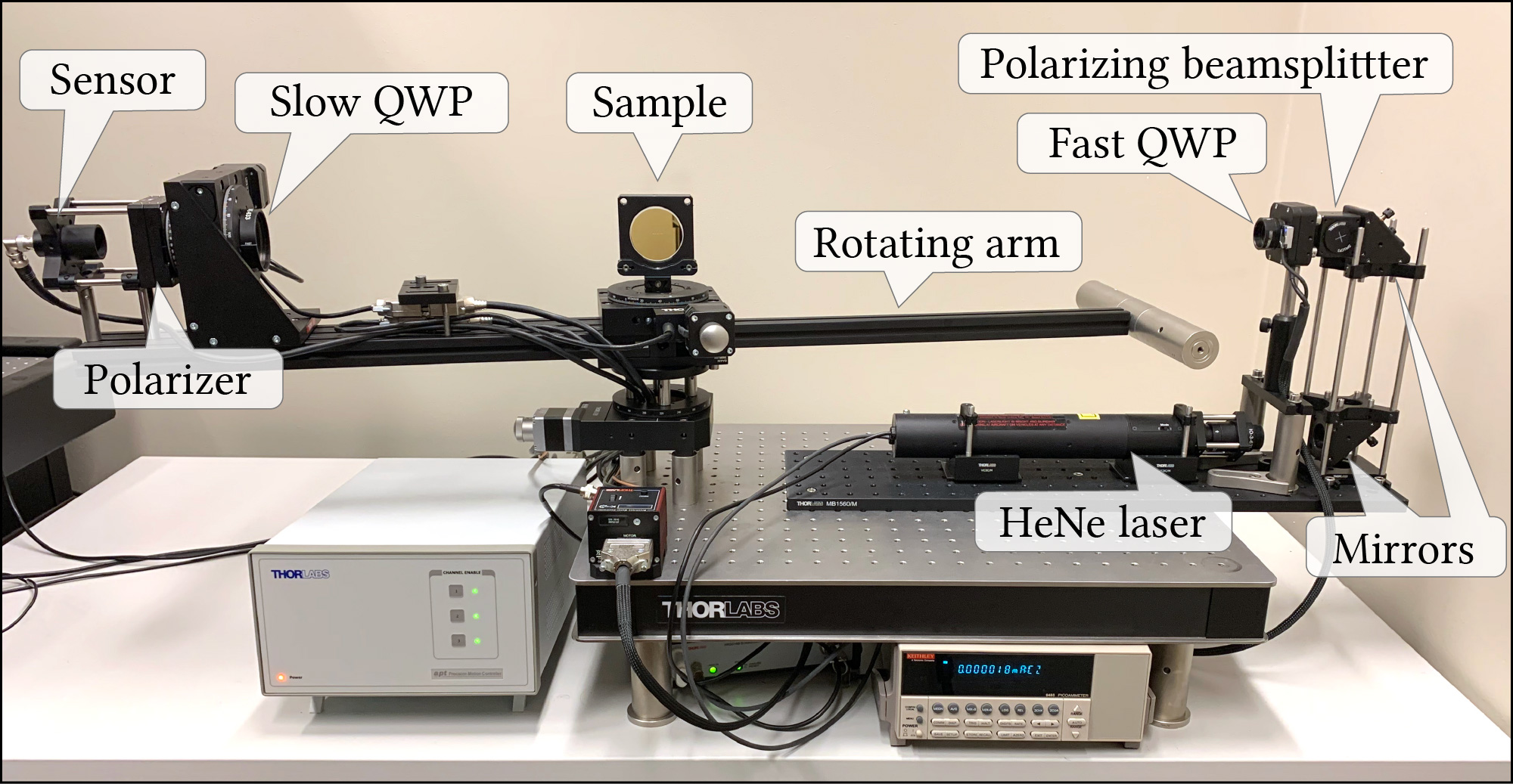
Both the sample and the analyzer module are mounted such that they can rotate independently of each other. This means, we can probe the same with any combination of incident and outgoing angles \(\theta_i\), \(\theta_o\). This video showcases the measurement process for a small set of these angles:

As part of the system calibration we first perform a measurement without any sample, effectively capturing the air and any potential inaccuracies of the device. As demonstrated in the following plot, the measured signal follows closely the expected curve from theory and hence the reconstructed Mueller matrix \(\mathbf{M}^{\text{air}}\) is very close to the identity:

\[\begin{split}\begin{equation} \mathbf{M}^{\text{air}} = \begin{bmatrix} 1.00048 & 0.04183 & -0.00323 & -0.00198 \\ 0.00466 & 1.03467 & -0.00114 & -0.01816 \\ -0.01167 & 0.00397 & 1.03684 & -0.00046 \\ 0.00007 & -0.00043 & 0.00172 & 0.99927 \end{bmatrix} \end{equation}\end{split}\]

For the actual measurements we then use \(\mathbf{M}^{\text{air}}\) as a correction term by multiplying its inverse:

\[\begin{equation} \mathbf{M}^{\text{final}} = (\mathbf{M}^{\text{air}})^{-1} \cdot \mathbf{M} \end{equation}\]

---

We measured two representative materials (conductor and dielectric) that can be accurately described by the Fresnel equations:

1. An unprotected gold mirror (M03).

2. An absorptive neutral density filter (NG1), made from Schott glass. This filter absorbs most of the refracted light and thus is very similar to observing only the reflection component of the Fresnel equations on dielectrics.

In the following we show the DRR signal (densely measured over all \(\theta_i = -\theta_o\) configurations of perfect specular reflection) and the reconstructed Mueller matrix entries compared to the analytical version from Mitsuba 3 (plotted over all \(\theta_i\) angles). Note that some areas (highlighted in gray) cannot be measured due to the sensor or sample holder blocking the light beam.

For readability, we only show the relevant Mueller matrix entries that are expected to be non-zero for the Fresnel equations:

\[\begin{split}\begin{equation} \begin{bmatrix} A & B & 0 & 0 \\ B & A & 0 & 0 \\ 0 & 0 & C & S1 \\ 0 & 0 & S2 & C \end{bmatrix} \end{equation}\end{split}\]

In both the conductor and dielectric case we observe excellent agreement between theory and captured data.

Gold (conductor)

Schott NG1 (dielectric)

Image-based measurements

We also compare against the gold measurement available in the pBRDF database acquired by Baek et al. [BZK+20]. In comparison to our setup that measures only the in-plane \(\theta_i, \theta_o\) angles, this data covers the full isotropic pBRDF but with lower accuracy. Nonetheless, the encoded Mueller matrices agree qualitatively with our implementation.

For details about this capture setup, please refer to the details given in the corresponding article.

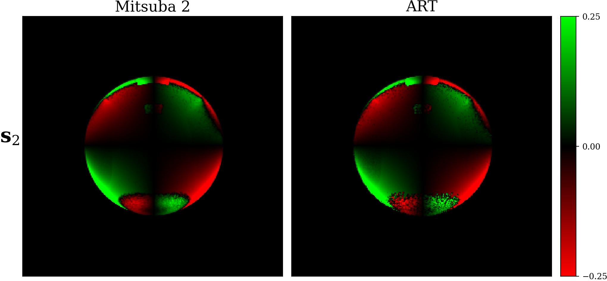
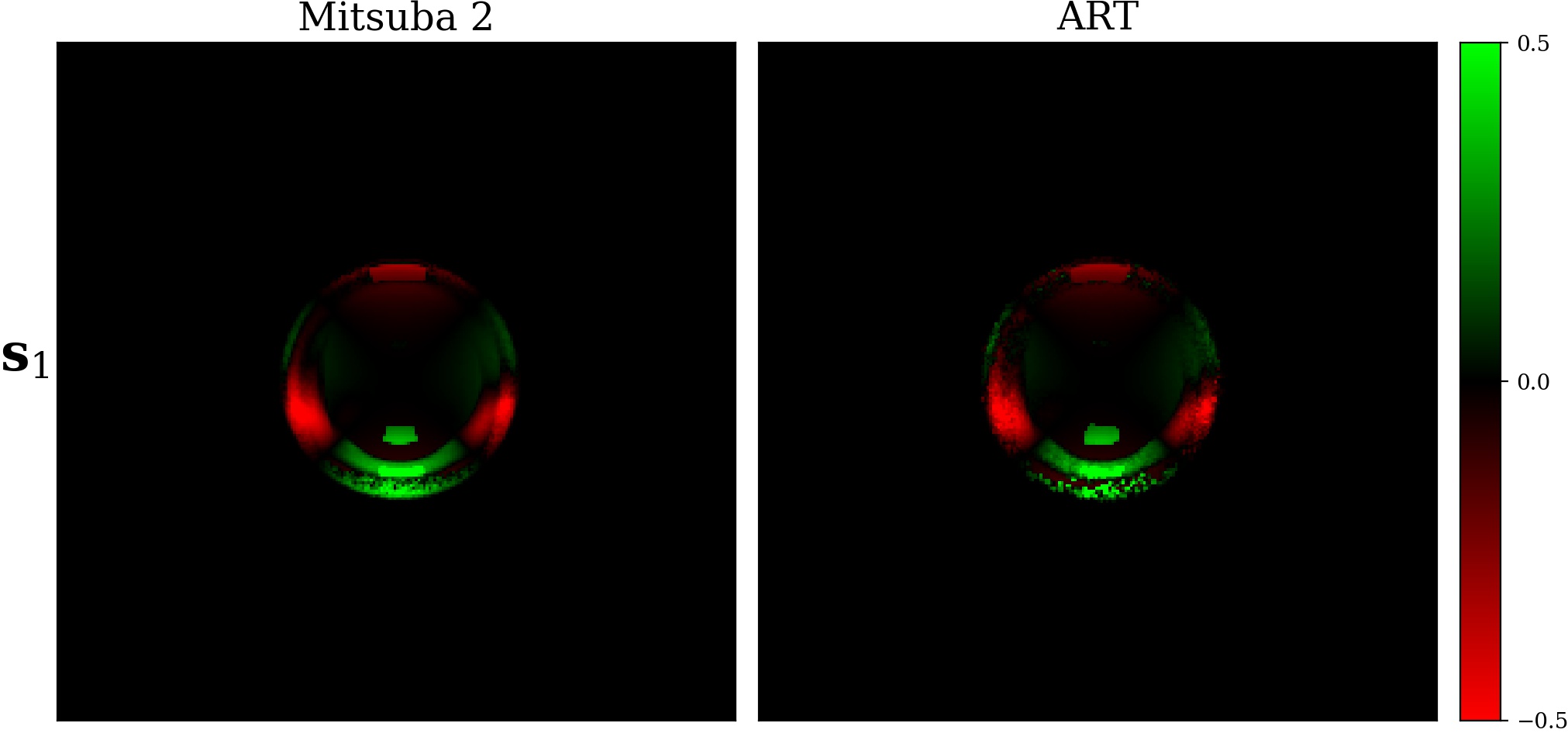
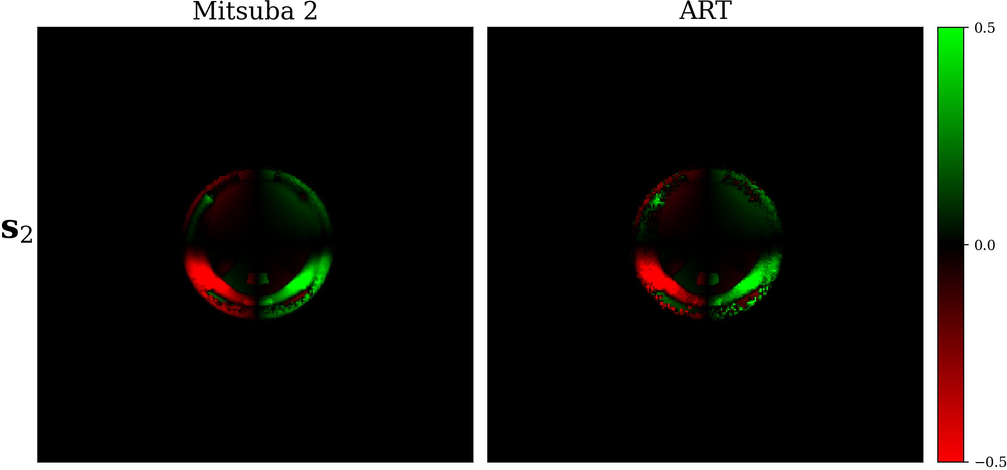
Validation against ART

Comparison

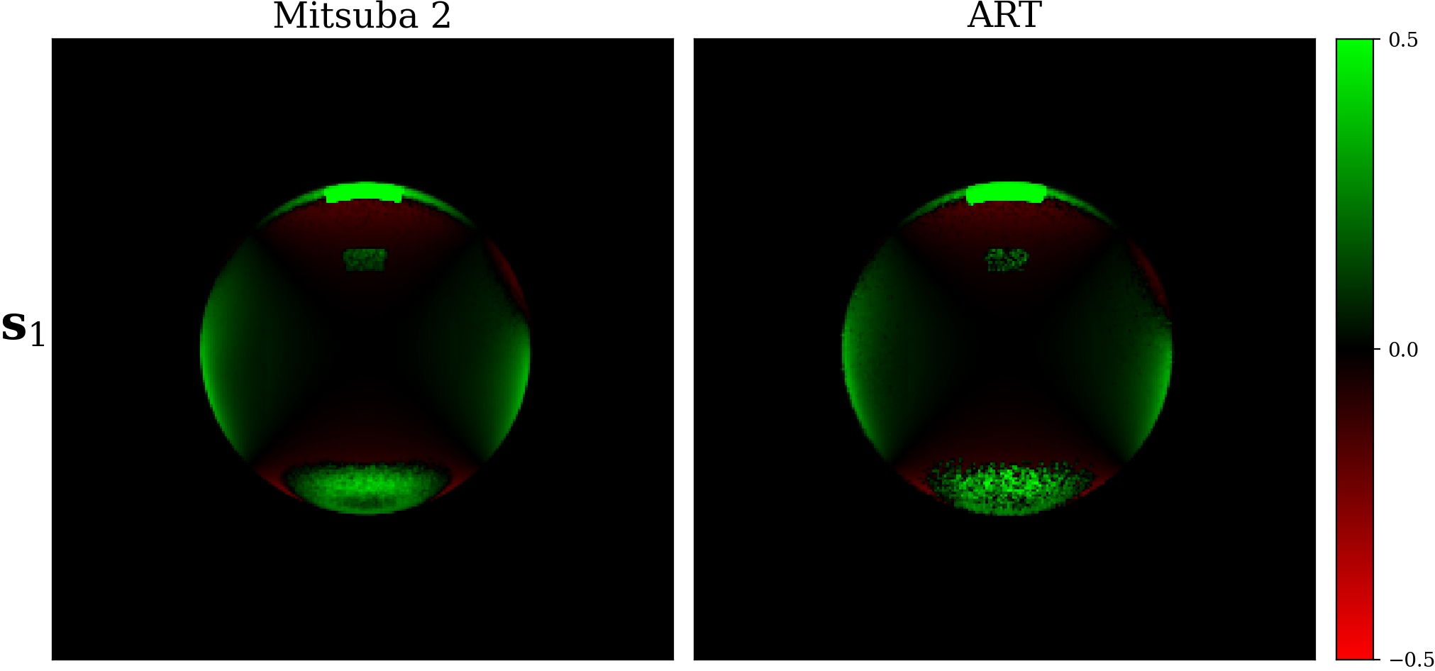
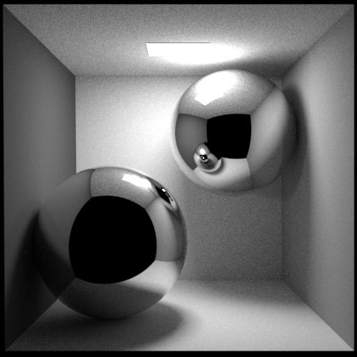
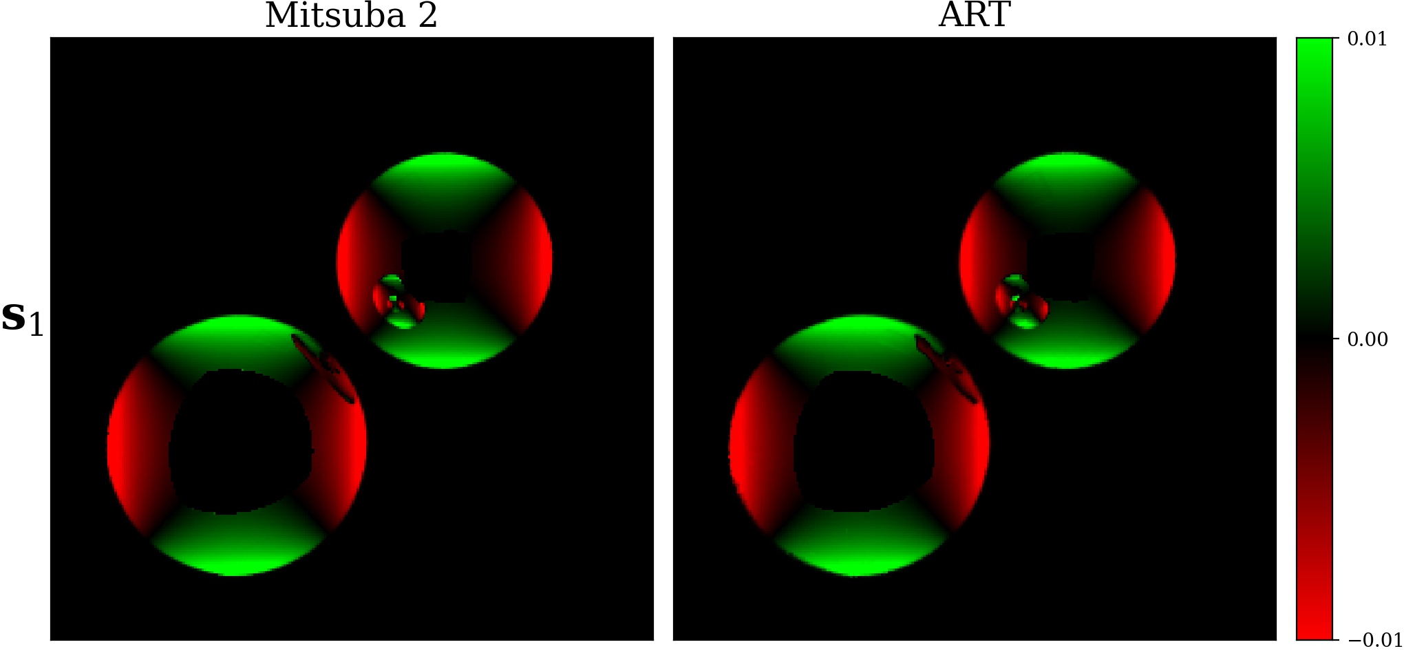
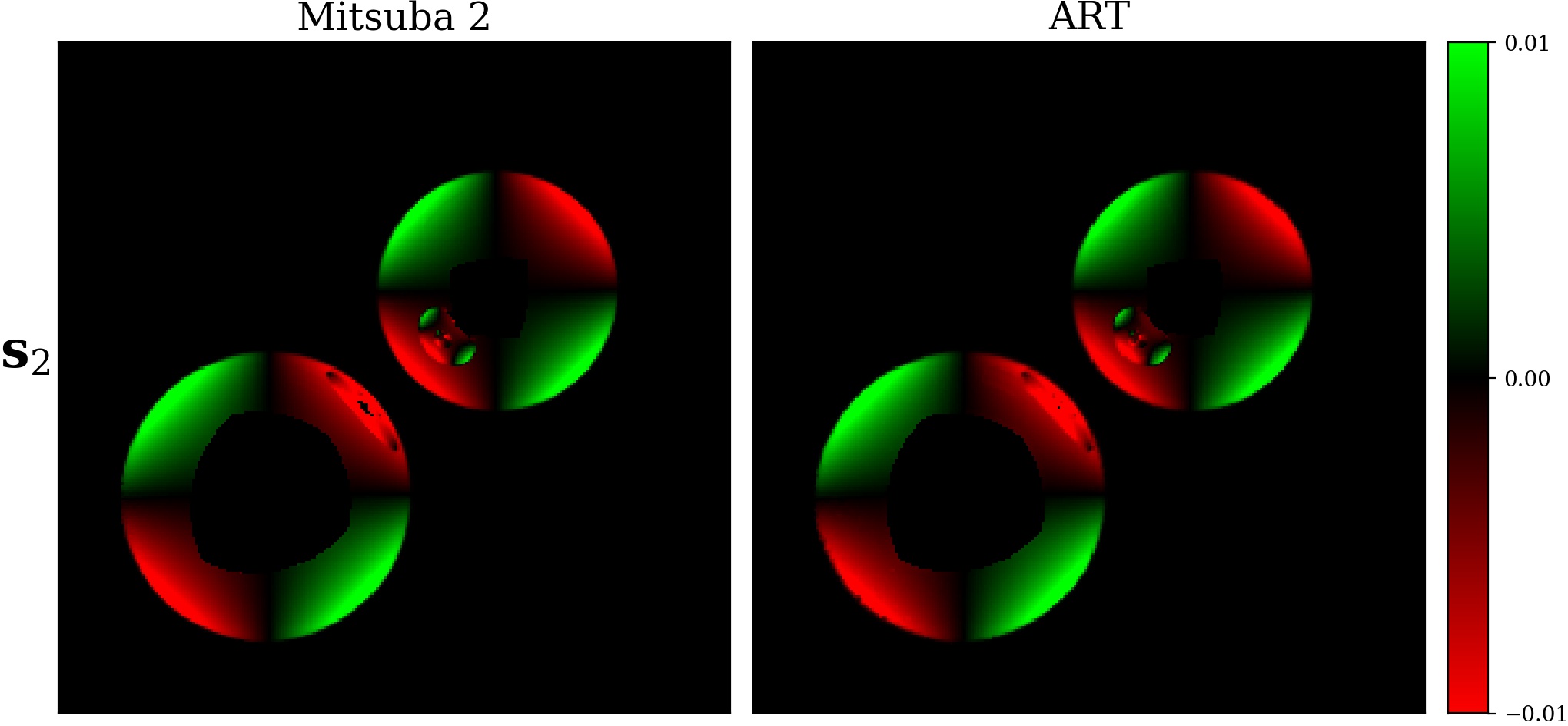
During development of Mitsuba 3 we also compared its polarized output against the existing implementation in the Advanced Rendering Toolkit (ART) research rendering system.

We used a few simple test scenes that we were able to reproduce in both systems that involve specular reflections and refractions. In each case, we directly compare the Stokes vector output (see also Section Stokes vector output) of the two systems. For ART, this information is normalized (s.t. \(\mathbf{s}_0 = 1\)) so we apply this consistently also to our results.

Dielectric reflection

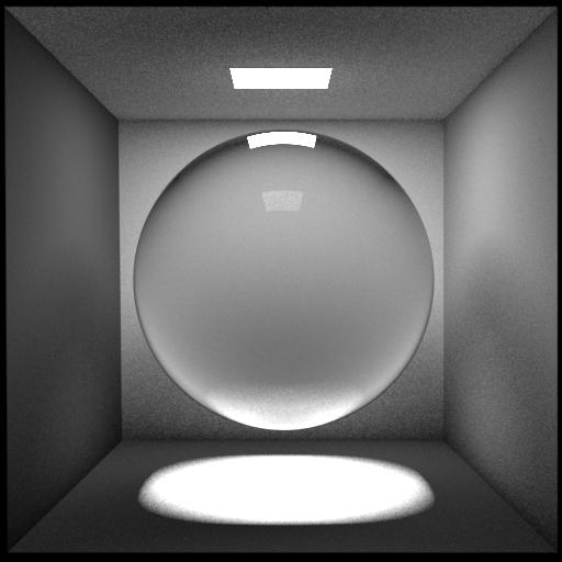
A simple Cornell box scene with a dielectric sphere (\(\eta = 1.5\)) that causes reflection and refraction.

Dielectric internal reflection

The same scene as before, but the IOR is reversed (\(\eta = 1/1.5\)) which causes internal reflection.

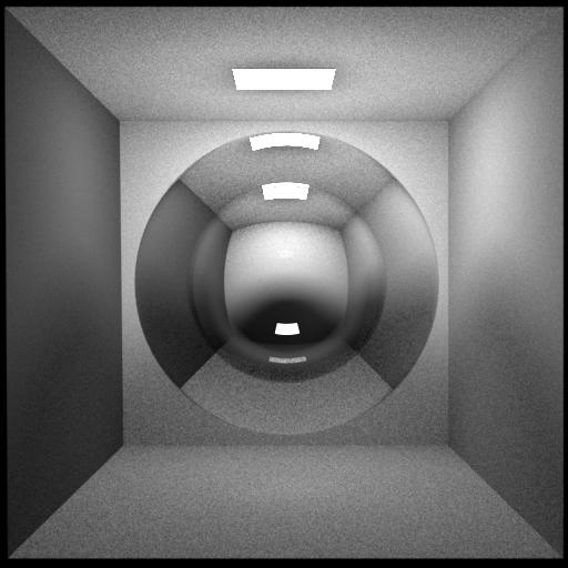
Conductor reflections

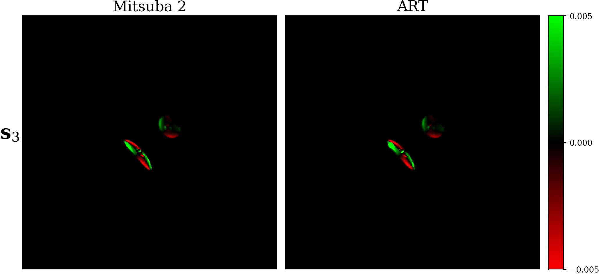
This scene uses two conductor spheres (\(\eta = 0.052 - 3.905 i\)) and also causes elliptical polarization due to the phase shifts and two-bounce reflections between the spheres.

Bugfix in ART

During the initial comparison, we discovered a subtle bug in ART’s implementation of the Fresnel equations. In their system, these are implemented based on an alternative formulation [WW12], originally from [WK90]:

\[\begin{split}\begin{align} F_{\bot} &= \frac{a^{2} + b^{2} - 2 a \cos\theta + \cos^{2}\theta}{a^{2} + b^{2} + 2 a \cos\theta + \cos^{2}\theta} \\ F_{\parallel} &= \frac{a^{2} + b^{2} - 2 a \sin\theta \tan\theta + \sin^{2}\theta \tan^{2}\theta}{a^{2} + b^{2} + 2 a \sin\theta \tan\theta + \sin^{2}\theta \tan^{2}\theta} F_{\bot} \\ \tan\delta_{\bot} &= \frac{2 b \cos\theta}{\cos^{2}\theta - a^{2} - b^{2}} \label{eq:art_fresenl_tan_s} \\ \tan\delta_{\parallel} &= \frac{2 \cos\theta \left[ (n^{2} - k^{2})b - 2 n k a \right]}{(n^{2} + k^{2})^{2} \cos^{2}\theta - a^{2} - b^{2}} \label{eq:art_fresenl_tan_p} \end{align}\end{split}\]

with

\[\begin{split}\begin{align} \eta = n + i k \\ 2 a^{2} &= \sqrt{(n^{2} - k^{2} - \sin^{2}\theta)^{2} + 4 n^{2}k^{2}} + n^{2} - k^{2} - \sin^{2}\theta \\ 2 b^{2} &= \sqrt{(n^{2} - k^{2} - \sin^{2}\theta)^{2} + 4 n^{2}k^{2}} - n^{2} + k^{2} + \sin^{2}\theta \end{align}\end{split}\]

The Mueller matrix then follows this shape

\[\begin{split}\begin{equation} \begin{bmatrix} A & B & 0 & 0 \\ B & A & 0 & 0 \\ 0 & 0 & C & S \\ 0 & 0 & -S & C \end{bmatrix} \end{equation}\end{split}\]

using

\[\begin{split}\begin{align} A &= \frac{F_{\bot} + F_{\parallel}}{2} \\ B &= \frac{F_{\bot} - F_{\parallel}}{2} \\ C &= \cos(\delta_{\bot} - \delta_{\parallel}) \cdot \sqrt{F_{\bot} \cdot F_{\parallel}} \\ S &= \sin(\delta_{\bot} - \delta_{\parallel}) \cdot \sqrt{F_{\bot} \cdot F_{\parallel}} \end{align}\end{split}\]

The phase shifts \(\delta_{\bot}\) and \(\delta_{\parallel}\) are recovered using the arctan2 function. Essentially this is similar to our formulation where we take the argument / angle of the complex reflection amplitudes (Eq. (19)).

Most programming environments (C++, NumPy, MATLAB, …) consistently use the notation \(\theta = \text{arctan2}(y, x)\) for computing \(\arctan(y/x)\) without ambiguities. However, the ART source code accidentally used a flipped argument order \(\text{arctan2}(x, y)\) that is found e.g. in Mathematica.

Such an issue is particularly subtle for the following reasons:

1. This only affects the sign / handedness of the circular polarization component, which is in most cases of relatively little importance.

2. Circular polarization only arises when light that is already polarized in some way undergoes an additional phase shift, e.g. by total internal reflection on a dielectric or simple reflection on a conductor. Specifically, a single specular reflection of unpolarized light will never produce circular polarization.

One case where this can be observed is our Conductor reflections test scene from above. We illustrate this sign flip by repeating the comparison of the relevant \(\mathbf{s}_3\) Stokes component in that scene — but with the previous flawed implementation.

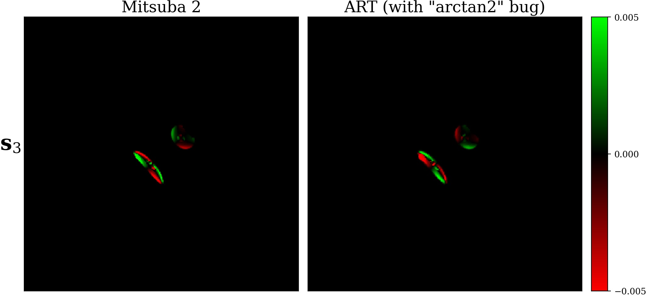
After communication with the authors of ART, this issue will be addressed in the next release.

Implementation

We now turn to the actual implementation of polarized rendering im Mitsuba 3. Due to its retargetable architecture, the whole system is already built on top of a templated Spectrum type and in principle it is very easy to use this mechanism to introduce the required Mueller/Stokes representations but some manual extra effort needs to be made to carefully place the correct Stokes coordinate system rotations. Implementing various forms of Mueller matrices (linear polarizers, retarders, Fresnel equations, …) covered in Section Mathematics of polarized light and Section Fresnel equations are also more or less straightforward and they can be found in the corresponding source file include/mitsuba/render/mueller.h.

As often is the case however, the devil lies in the details and throughout the development we ran into various issues related to coordinate systems and sign flips. In hindsight, these can all be attributed to mixing conventions from different sources [Muller69] or misconceptions about what they mean.

We briefly list these here for reference and to help people avoid these issues in the future:

1. We initially found it natural to track the Stokes reference frames (Section Reference frames) from the viewpoint of the light source. After a lot of confusion about the commonly used rotation matrices (Section Rotation of Stokes vector frames) and the meaning of left/right handed circular polarization we realized that almost all optics sources defines this reference frame the other way around, using the point of view of the sensor.

2. The “\(\bot\)” and “\(\parallel\)” components of the transverse wave (Section Theory) used in the Fresnel equations (i.e. perpendicular or parallel to the plane of incidence) are pretty clearly defined but we initially did not correctly interpret how these map to the Mueller-Stokes calculus. In particular, we (wrongly) assumed that the “\(\parallel\)” direction should be the “horizontal” axis of the incident and outgoing Stokes vectors. We discovered this issue after the measurements of a few representative materials (Section Validation against measurements) which could not be explained in any other way. The fact that “\(\bot\)” corresponds to the “horizontal” axis is also clear when taking a closer look at how the Fresnel equations are actually converted into Mueller matrices [Col71]. Surprisingly, this discussion is missing in many sources that include these matrices.

3. We were surprised to find that the complex index of refraction of conductors is most commonly defined with a negative imaginary component, i.e. \(\eta = n - k i\) (Section Equations). In contrast, the usual definition in computer graphics uses a positive sign (\(\eta = n + k i\)) [PJH16]. (In fact, both signs produce the same outcome if we assume no polarized light.) This is also a point where our measurements (Section Validation against measurements) were really useful. As the Fresnel equations need to behave consistently between dielectrics (\(k = 0\)) and conductors (\(k > 0\)), another good validation was to make sure there is no sudden sign flip between a dielectric (e.g. \(\eta = 1.5\)) and a conductor with only a tiny amount of extinction (e.g. \(\eta = 1.5 - 0.0001 i\)).

4. One of the biggest confusions we faced is related to the Fresnel equations themselves (Section Different conventions in the literature and Section Different conventions in the context of Mueller matrices). For instance, the Fresnel or Verdet conventions of defining the underlying electric fields cause subtle sign flips in some of the equations. You can also define phase shifts (e.g. on total internal reflection) as either phase retardations or advances. Again, this only flips a few signs but together this gives a few different combinations of signs in the resulting Mueller matrices (e.g. Eq. (30)) — and you can find all of them in various sources. All of them are correct (in their respective conventions) but this situation makes it very hard to work with multiple references simultaneously.

We originally used Stellar polarimetry [Cla09] as our main sources so our implementation was consistent from the beginning. However the formulation there uses the Fresnel convention and phase delays and we did not initially understand why most other sources we looked had things written down differently. (And we always came back to this question whenever some other part of the implementation was not behaving as expected.) Towards the end of development (when we had consistency with the measurements) and after a thorough literature review we decided to switch Mitsuba 3 to the much more common Verdet convention and phase advances.

The remainder of this document serves as an overview of all relevant parts of the code base and it will hopefully be useful for both understanding and extending the polarization specific aspects of Mitsuba 3.

Representation

Stokes and Mueller types

Using the Mueller-Stokes calculus (Section Mathematics of polarized light) in a renderer introduces a type mismatch between fundamental quantities used in different parts of the system. For instance, the Spectrum array type (with either a single monochromatic entry, 3 RGB values, or intensities at sampled wavelengths) would normally be used to represent emission, reflectance, and importance in non-polarized renderers. Polarization requires us to change it to Stokes vectors in the former case, and Mueller matrices in the latter two cases however.

We avoid this asymmetry we made the decision to only use Mueller matrices where in the case of Stokes vectors, only the first column is non-zero:

This leads to some unnecessary arithmetic but simplifies the API which is especially useful when implementing bidirectional techniques. In particular, Mitsuba 3 has a single API (include/mitsuba/render/endpoint.h) that is shared by both emitters and sensors.

---

When also considering the different color representations in Mitsuba 3 there are three possible Mueller matrix types:

1. Monochrome mode: \(4 \times 4 \times 1\) matrices.

This mode completely disables all concept of color in Mitsuba 3, and instead, only the intensity / luminance of light is simulated.

Example: scalar_mono_polarized.

2. RGB mode: \(4 \times 4 \times 3\) matrices

RGB colors are used in many rendering systems for its simplicity. However it can be a poor approximation of how color actually works. The accuracy is even more questionable in polarized rendering modes, as e.g. the Fresnel equations for conductors will not be evaluated at wavelengths with actual physical meaning.

Example: scalar_rgb_polarized.

3. Spectral mode: \(4 \times 4 \times 4\) matrices

A full spectral color representation is the recommended approach to use for polarized rendering. The last dimension is \(4\) because Mitsuba 3 by default traces four randomly sampled wavelengths at once.

Example: scalar_spectral_polarized.

---

The remainder of this section covers a few more implementation details / helpful functions involving the Spectrum type and polarization.

1. There is a type trait to detect whether the Spectrum type is polarized or not that can be used for code blocks that are only needed in polarized variants. This is especially helpful in conjunction with the C++17 constexpr feature:

// From `include/mitsuba/core/traits.h`
template <typename T> constexpr bool is_polarized_v = ...

// Example use case
if constexpr (is_polarized_v<Spectrum>) {
    // ... only compiled in polarized modes ...
}

2. There is a similar type trait to turn a polarized Spectrum (i.e. a matrix) into an unpolarized form (i.e. only a 1D/3D/4D vector depending on the underlying color representation).

This is useful for instance when querying reflectance data from a bitmap texture where no polarization specific information is stored.

// From `include/mitsuba/core/traits.h`
template <typename T> using unpolarized_spectrum_t = ...

// Example use case
using UnpolarizedSpectrum = unpolarized_spectrum_t<Spectrum>;

3. There exists a helper function to extract the \((1, 1)\) entry of the Mueller matrix / Stokes vector. Essentially, it will turn any Spectrum value into an UnpolarizedSpectrum.

This is used in a few places in the renderer where we do not care about the additional polarization information tracked by the Mueller matrix. For instance, when performing Russian Roulette (stochastic termination of long light paths) based on the current path throughput or when writing a final RGB pixel value to the image, see Section Rendering output.

// From `include/mitsuba/core/spectrum.h`

template <typename T>
unpolarized_spectrum_t<T> unpolarized_spectrum(const T& s) {
    if constexpr (is_polarized_v<T>) {
        // First entry of the Mueller matrix is the unpolarized spectrum
        return s(0, 0);
    } else {
        return s;
    }
}

4. Another helper function returns a depolarizing Mueller matrix (with only its \((1, 1)\) entry used) where the input is usually an UnpolarizedSpectrum value.

This is obviously used in places where we want materials to act as depolarizers, e.g. in the case of a Lambertian diffuse material. However, there are also many BSDFs where it is currently not clear how they should interact with polarized light, or the functionality is not yet implemented. For now, these all act as depolarizers. Lastly, this is also used for light sources, as they currently all emit completely unpolarized light in Mitsuba 3.

// From `include/mitsuba/core/spectrum.h`

template <typename T>
auto depolarizer(const T &s = T(1)) {
    if constexpr (is_polarized_v<T>) {
        T result = dr::zero<T>();
        result(0, 0) = s(0, 0);
        return result;
    } else {
        return s;
    }
}

// Example use case, where the value returned from the texture is of type
// `UnpolarizedSpectrum`.
Spectrum s = depolarizer<Spectrum>(m_texture->eval(si, active));

Coordinate frames

A second complication of the Mueller-Stokes calculus is the need to keep track of reference frames throughout the rendering process. One choice (e.g. used by the ART rendering system) would be to store incident and outgoing frames with each Mueller matrix type directly (where one of the two is redundant in case the matrix encodes a Stokes vector).

To better leverage the retargetable design of Mitsuba 3 where the Spectrum template type is substituted for arrays of varying dimensions we chose to instead represent these coordinate systems implicitly. For each unit vector, we can construct its orthogonal Stokes basis vector:

Constructing a unique Stokes basis vector for the given unit vector.

// From `include/mitsuba/render/mueller.h`
template <typename Vector3>
Vector3 stokes_basis(const Vector3 &omega) {
    return coordinate_system(omega).first;
}

Here, the coordinate_system function constructs two orthogonal vectors to omega in a deterministic way [DBC+17]. The resulting Stokes basis vector is therefore always unique for a given direction.

Recall from Section Mueller matrices that whenever two Mueller matrices (or a Mueller matrix and a Stokes vector) are multiplied with each other, their respective outgoing and incident reference frames need to be aligned with each other. This is usually achieved by some combination of rotator matrices (Eq. (3)) that transform the Stokes frames (Section Rotation of Stokes vector frames). Mitsuba 3 implements two versions where the rotation angle \(\theta\) is either directly known, or inferred from a provided set of basis vectors before and after the desired rotation:

Rotate Stokes vector reference frames.

// From `include/mitsuba/render/mueller.h`

// Construct the Mueller matrix that rotates the reference frame of a Stokes
// vector by an angle `theta`.
template <typename Float>
MuellerMatrix<Float> rotator(Float theta) {
    auto [s, c] = dr::sincos(2.f * theta);
    return MuellerMatrix<Float>(
        1, 0, 0, 0,
        0, c, s, 0,
        0, -s, c, 0,
        0, 0, 0, 1
    );
}

// Construct the Mueller matrix that rotates the reference frame of a Stokes
// vector from `basis_current` to `basis_target`.
// The masked condition ensures that rotation is performed in the right direction.
template <typename Vector3,
          typename Float = dr::value_t<Vector3>,
          typename MuellerMatrix = MuellerMatrix<Float>>
MuellerMatrix rotate_stokes_basis(const Vector3 &forward,
                                  const Vector3 &basis_current,
                                  const Vector3 &basis_target) {
    Float theta = unit_angle(dr::normalize(basis_current),
                             dr::normalize(basis_target));

    auto flip = dr::dot(forward, dr::cross(basis_current, basis_target)) < 0;
    dr::masked(theta, flip) *= -1.f;
    return rotator(theta);
}

We then have more functions that build on top of this to cover the common cases of rotating incident/outgoing Mueller reference frames (left, see Section Rotation of Mueller matrix frames) and rotated optical elements (right, see Section Rotation of optical elements):

Rotate Mueller matrix reference frames.

// From `include/mitsuba/render/mueller.h`

// "Rotate" a Mueller matrix in the general case (i.e. when both
// sides use a different basis).
//
// Before:
//     Matrix M operates from `in_basis_current` to `out_basis_current` frames.
// After:
//     Returned matrix operates from `in_basis_target` to `out_basis_target` frames.
template <typename Vector3,
          typename Float = dr::value_t<Vector3>,
          typename MuellerMatrix = MuellerMatrix<Float>>
MuellerMatrix rotate_mueller_basis(const MuellerMatrix &M,
                                   const Vector3 &in_forward,
                                   const Vector3 &in_basis_current,
                                   const Vector3 &in_basis_target,
                                   const Vector3 &out_forward,
                                   const Vector3 &out_basis_current,
                                   const Vector3 &out_basis_target) {
    MuellerMatrix R_in  = rotate_stokes_basis(in_forward,
                                              in_basis_current,
                                              in_basis_target);
    MuellerMatrix R_out = rotate_stokes_basis(out_forward,
                                              out_basis_current,
                                              out_basis_target);
    return R_out * M * transpose(R_in);
}

// Special case of `rotate_mueller_basis`.
// "Rotate" a Mueller matrix in the case of collinear incident and
// outgoing directions (i.e. when both sides have the same basis).
//
// Before:
//     Matrix M operates from `basis_current` to `basis_current` frames.
// After:
//     Returned matrix operates from `basis_target` to `basis_target` frames.
template <typename Vector3,
          typename Float = dr::value_t<Vector3>,
          typename MuellerMatrix = MuellerMatrix<Float>>
MuellerMatrix rotate_mueller_basis_collinear(const MuellerMatrix &M,
                                             const Vector3 &forward,
                                             const Vector3 &basis_current,
                                             const Vector3 &basis_target) {
    MuellerMatrix R = rotate_stokes_basis(forward, basis_current, basis_target);
    return R * M * transpose(R);
}

// Apply a rotation to the Mueller matrix of a given optical element.
template <typename Float>
MuellerMatrix<Float> rotated_element(Float theta,
                                     const MuellerMatrix<Float> &M) {
    MuellerMatrix<Float> R = rotator(theta), Rt = transpose(R);
    return Rt * M * R;
}

Both of these require a forward unit vector that points along the propagation direction of light.

Algorithms and materials

With the discussion about representation of light via Stokes vectors and scattering via Mueller matrices out of the way we can now turn to the more rendering specific aspects of the implementation: the algorithms, material models, and how the two are coupled.

Handling of light paths

In principle, not much changes when adding polarization to a rendering algorithm and the retargetable type system of Mitsuba 3 will do a lot of the heavy lifting. In particular, emitters will return emission in form of Stokes vectors (or rather Mueller matrices with three zero valued columns.) and polarized bidirectional scattering distribution functions (pBSDFs) will return Mueller matrices that are multiplied with the emission:

As it turns out, polarization breaks some of the symmetry of light transport that is usually exploited by rendering algorithms [MSWK16], [JA18], especially for bidirectional techniques. As a consequence, the actual direction of light propagation (i.e. from emitter to sensor) needs to be kept in mind at all times as it dictates the ordering in which matrices will be multiplied.

---

Consider the two extreme ends of bidirectional algorithms that construct a light path with \(n\) vertices \((\mathbf{x}_0, \dots, \mathbf{x}_{n-1}\)) where the ordering is from emitter to sensor as in the figure above:

1. Light tracing follows the natural ordering of events: we sample rays starting from light sources and their emitted light (in form of a Stokes vector \(\mathbf{s}_0\)) is multiplied by Mueller matrices \(\mathbf{M}_k\) returned from pBSDFs encountered along all scattering events \(k\) of a light path.

During path generation, a throughput variable \(\boldsymbol{\beta}_k^{\text{(lt)}}\) is updated which is the sequence of previous Mueller matrices multiplied onto the original emission vector from the left:

\[\boldsymbol{\beta}_k^{\text{(lt)}} = \mathbf{M}_k \cdot \mathbf{M}_{k-1} \cdot \dots \cdot \mathbf{M}_1 \cdot \mathbf{s}_0\]

2. Path tracing, on the other hand, follows things in reverse: rays are sampled starting from the sensor side. As conceptually the same computation needs to take place as in the previous case, the path throughput at each bounce is now a Mueller matrix \(\mathbf{B}_k^{\text{(pt)}}\) where Mueller matrices from encountered pBSDFs are multiplied from the right:

\[\mathbf{B}_k^{\text{(pt)}} = \mathbf{M}_{n-1} \cdot \mathbf{M}_{n-2} \cdot \dots \cdot \mathbf{M}_k\]

Only when hitting the light source (vertex \(k=0\)) directly, or connecting to it via next event estimation will the Stokes vector \(\mathbf{s}_0\) be actually multiplied as well.

---

Polarized rendering algorithms compute Stokes vectors as output where either only their intensity (1st entry) or all individual components are written into some image format, see Section Rendering output below.

pBSDF evaluation and sampling

During Section Handling of light paths we glossed over the tricky question of coordinate system rotations and silently assumed that all Mueller matrix multiplications are taking place in their valid reference frames. Mitsuba 3 deals with this issue in a consistent way that is tightly coupled to how BSDF evaluations and sampling take place.

Default case without polarization

For completeness, we will first briefly discuss the usual convention without polarization specific changes. Also see include/mitsuba/render/bsdf.h for details about the BSDF API.

Mitsuba 3 (like most modern rendering systems) uses BSDF implementations that are completely decoupled from the actual rendering algorithms in order to be as extensible as possible. To facilitate this, their sampling and evaluation is taking place in some canonical local coordinate system that is always aligned with the shading normal \(\mathbf{n}\) pointing up (towards \(+\mathbf{z}\)):

Note also how both incident and outgoing directions \(\boldsymbol{\omega}_i, \boldsymbol{\omega}_o\) point “away” from the center and that, due to reciprocity of BSDFs, they are completely interchangeable Care only needs to be taken when sampling the BSDFs, i.e. when only one direction is given initially, and a new one should be generated. In this scenario, Mitsuba 3 (arbitrarily) has the convention that \(\boldsymbol{\omega}_i\) is given, and \(\boldsymbol{\omega}_o\) is newly sampled.

As rendering algorithms take place in world space however, some transformations between the two spaces are necessary:

``to_local`` and ``to_world`` space transformations.

// From `include/mitsuba/core/frame.h`

// Convert from world coordinates to local coordinates
// with orthogonal frame `(s, t, n)`.
Vector3f to_local(const Vector3f &v) const {
    return Vector3f(dr::dot(v, s), dr::dot(v, t), dr::dot(v, n));
}

// Convert from local coordinates with orthogonal
// frame `(s, t, n)` to world coordinates.
Vector3f to_world(const Vector3f &v) const {
    return s * v.x() + t * v.y() + n * v.z();
}

Extra considerations with polarization

In a setting with polarization this aspect becomes more involved as there are now also Stokes basis vectors associated with the local & world space incident and outgoing directions that are subject to these transformations:

Mitsuba 3 makes heavy use of its implicit Stokes coordinate frames (Section Coordinate frames) here. Mueller matrices returned from pBSDF evaluation or sampling are always assumed to be valid for the implicit bases of the local unit vectors (\(-\boldsymbol{\omega}_o^{\text{local}}\) and \(\boldsymbol{\omega}_i^{\text{local}}\) in the Figure above). Or outlined more clearly in code:

BSDFContext ctx;                // Used to pass optional flags to BSDFs
SurfaceInteraction3f si = ...;  // Returned from ray-scene intersections.

// Incident and outgoing directions in world space
Vector3f wo = ...;
Vector3f wi = ...;

// Transform into local space ...
Vector3f wo_local = si.to_local(wo);
si.wi = si.to_local(wi);

// ... and evaluate the pBSDF.
Spectrum bsdf_val = bsdf->eval(ctx, si, wo_local);

// The returned Mueller matrix `bsdf_val` is then valid for the
// following input & output Stokes reference bases that are defined
// implicitly.
Vector3f bo_local = stokes_basis(-wo_local);
Vector3f bi_local = stokes_basis(si.wi);

In order to perform the correct rotations, throughout this description the two unit vectors need to point along the propagation direction of light. In practice, this means that compared to the unpolarized Figure above, the vector pointing towards the emitter side needs to be reversed.

At this point we have all the information to transform the Mueller matrix such that it is valid in the global Stokes bases bo = stokes_basis(-wo) and bi = stokes_basis(wi) where it can be safely multiplied as discussed in Section Handling of light paths earlier. This involves converting these basis into a common space and applying a Mueller matrix rotation (Section Coordinate frames). All of this is done as part of a single helper function:

``to_world_mueller`` space transformations for Mueller matrices.

// From `include/mitsuba/render/interaction.h`

// Transform a Mueller matrix `M_local` that is the result of evaluating or sampling
// a pBSDF in local space to world space.
// `in_forward_local` and `out_forward_local` are the unit vectors (also in local
// space) that point along the light propagation direction before and after the
// scattering event.
Spectrum to_world_mueller(const Spectrum &M_local,
                          const Vector3f &in_forward_local,
                          const Vector3f &out_forward_local) const {
    if constexpr (is_polarized_v<Spectrum>) {
        // Incident and outgoing directions are transformed into world space
        Vector3f in_forward_world  = to_world(in_forward_local),
                 out_forward_world = to_world(out_forward_local);

        // Establish the "current" and "target" incident basis:
        //     "current": The implicit basis of the local-space incident
                          direction, transformed into world space.
        //     "target":  The implicit basis of the world-space incident direction.
        Vector3f in_basis_current = to_world(mueller::stokes_basis(in_forward_local)),
                 in_basis_target  = mueller::stokes_basis(in_forward_world);

        // Analogously establish the same for the outgoing direction.
        Vector3f out_basis_current = to_world(mueller::stokes_basis(out_forward_local)),
                 out_basis_target  = mueller::stokes_basis(out_forward_world);

        // Rotate the Mueller matrix frames to transform correctly between the two.
        return mueller::rotate_mueller_basis(M_local,
                                             in_forward_world, in_basis_current, in_basis_target,
                                             out_forward_world, out_basis_current, out_basis_target);
    } else {
        // No-op in unpolarized variants.
        return M_local;
    }

The complementary to_local_mueller function is also implemented but is usually not needed apart from debugging purposes.

Finally, the following two code snippets show heavily commented pBSDF evaluation and sampling steps that include all of the considerations above. This is comparable to what is done e.g. in the current path tracer implementation of Mitsuba 3 (src/integrators/path.cpp). Note that only the lines involving to_world_mueller had to be added compared to a standard unpolarized path tracer.

Evaluate a pBSDF

BSDFContext ctx;                // Used to pass optional flags to BSDFs
SurfaceInteraction3f si = ...;  // Returned from ray-scene intersections.

// Incident and outgoing directions in world space
Vector3f wo = ...;
Vector3f wi = ...;

// Transform into local space ...
Vector3f wo_local = si.to_local(wo);
si.wi = si.to_local(wi);

// ... and evaluate the BSDF
Spectrum bsdf_val = bsdf->eval(ctx, si, wo_local);

// At this point, the Mueller matrix `bsdf_val` is valid in the implicit
// reference frames of local space vectors `-wo_local` and `si.wi`.
// Both unit vectors follow the direction of the light. (We assume an
// algorithm similar to path tracing here. When tracing from the emitter side,
// things will be reversed.)

// Transform Mueller matrix into world space
bsdf_val = si.to_world_mueller(bsdf_val, -wo_local, si.wi);

// Now, the Mueller matrix `bsdf_val` is valid in the implicit
// reference frames of world space vectors `-wo` and `wi`.

Sample from a pBSDF

BSDFContext ctx;
SurfaceInteraction3f si = ...;

// Incident direction in world space ...
Vector3f wi = ...;
// ... and transformed into local space
si.wi = si.to_local(wi);

// Sample based on random numbers (in local space)
auto [bs, bsdf_weight] = bsdf->sample(ctx, sampler.next_1d(), sampler.next_2d());

// At this point, the Mueller matrix `bsdf_weight` is valid in the implicit
// reference frames of local space vectors `-bs.wo` and `si.wi`.
// Both unit vectors follow the direction of the light. (We assume an
// algorithm similar to path tracing here. When tracing from the emitter side,
// things will be reversed.)

// Transform sampled direction into world space
Vector3f wo = si.to_world(bs.wo);

// Transform Mueller matrix into world space
bsdf_weight = si.to_world_mueller(bsdf_weight, -bs.wo, si.wi);

// Now, the Mueller matrix `bsdf_weight` is valid in the implicit
// reference frames of world space vectors `-wo` and `wi`.

Implementing pBSDFs

After looking at rendering algorithms and how they interact with pBSDFs, we still need to discuss the internals of a given pBSDF implementation, i.e. what is happening in the (local space) evaluation and sampling routines.

As mentioned above, these should always return valid Mueller matrices based on the implicit reference frames of the (local) incident and outgoing directions. In the following Figure, these are marked as \(\mathbf{b}_o^{\text{local}}\) and \(\mathbf{b}_i^{\text{local}}\).

In terms of code, they are computed as

Vector3f bo_local = stokes_basis(-wo_local);
Vector3f bi_local = stokes_basis(wi_local);

When pBSDFs construct Mueller matrices, these are usually based on some very specific Stokes basis convention, e.g. described in textbooks. For instance, the current pBSDFs found in Mitsuba 3 are mostly built from Mueller matrices based on the Fresnel equations. This means, they are constructed based on the perpendicular (”\(\bot\)”) and parallel (”\(\parallel\)”) vectors relative to the plane of reflection. Please refer back to Section Fresnel equations for details. In particular, the main “horizontal” or \(\mathbf{b}_{i/o}\) vector is the “\(\bot\)” component that can be constructed as follows for incident and outgoing directions:

Vector3f n(0, 0, 1);  // Surface normal
Vector3f s_axis_in  = dr::normalize(dr::cross(n, -wo_local)),
         s_axis_out = dr::normalize(dr::cross(n, wi_local));

As illustrated in the Figure above, a (final) coordinate rotation needs to take place to convert the Mueller matrix to the right bases before it can be returned from the pBSDF.

For this rotation, we need to know along what direction the light is traveling so we need to correctly distinguish between \(\boldsymbol{\omega}_i\) and \(\boldsymbol{\omega}_o\). During path tracing (or any algorithm that traces from the sensor side), Mitsuba 3 uses BSDFs with the convention that light arrives from \(-\boldsymbol{\omega}_o\) and leaves along \(\boldsymbol{\omega}_i\) (because \(\boldsymbol{\omega}_o\) is sampled based on \(\boldsymbol{\omega}_i\) that points towards the sensor side). During light tracing from emitters, the roles are reversed however: light arrives from \(-\boldsymbol{\omega}_i\) and leaves along \(\boldsymbol{\omega}_o\). Mitsuba 3 has a special BSDF flag (TransportMode) that carries the relevant information to resolve this confusion and is used for similar “non-reciprocal” situations in bi-directional techniques [Vea98].

Putting everything together, here is a short snippet as example of how the a pBSDF evaluation based on the Fresnel equations can be implemented. This is very close to what is done for instance in src/bsdfs/conductor.cpp.

Example pBSDF evaluation based on Fresnel equations.

// Incident and outgoing directions, given in local space.
Vector3f wo_local = ...;
Vector3f wi_local = ...;

// Due to the coordinate system rotations for polarization-aware
// pBSDFs below we need to know the propagation direction of light.
// In the following, light arrives along `-wo_hat` and leaves along
// `+wi_hat`.
//
// `TransportMode` has two states:
//     - `Radiance`, meaning we trace from the sensor to the light sources
//     - `Importance`, meaning we trace from the light sources to the sensor
//
Vector3f wo_hat = ctx.mode == TransportMode::Radiance ? wo_local : wi_local,
         wi_hat = ctx.mode == TransportMode::Radiance ? wi_local : wo_local;

// Querty the complex index of refraction
dr::Complex<UnpolarizedSpectrum> eta = ...;

// Evaluate the Mueller matrix for specular reflection.
// This will internally call the Fresnel equations and assemble the correct
// matrix.
// The incident angle cosine is cast to `UnpolarizedSpectrum` to be compatible with
// `eta` when calling the function.
UnpolarizedSpectrum cos_theta = Frame3f::cos_theta(wo_hat);
Spectrum value = mueller::specular_reflection(cos_theta, eta);

// Apply the "handedness change" Mueller matrix that is necessary for reflections.
// Recall from the Section about Fresnel equations that this is a diagonal matrix
// with entries [1, 1, -1, -1].
value = mueller::reverse(value);

// Compute the Stokes reference frame vectors of this matrix that are
// perpendicular to the plane of reflection.
Vector3f n(0, 0, 1);
Vector3f s_axis_in  = dr::normalize(dr::cross(n, -wo_hat)),
         s_axis_out = dr::normalize(dr::cross(n, wi_hat));

// Rotate in/out reference vector of `value` s.t. it aligns with the implicit
// Stokes bases of -wo_hat & wi_hat. */
value = mueller::rotate_mueller_basis(value,
                                      -wo_hat, s_axis_in, mueller::stokes_basis(-wo_hat),
                                       wi_hat, s_axis_out, mueller::stokes_basis(wi_hat));

Rendering output

In this section we will briefly discuss the output side of the rendering system and how to extract polarization specific information from it to use in experiments.

Intensity output

In most natural scenes, polarization effects are very subtle and hardly visible to the eye. Enabling polarized rendering modes in Mitsuba 3 therefore also usually does not produce vastly different outputs compared to an unpolarized mode. However, in particular cases such as specular interreflections or as soon as polarizing optical elements (such as linear polarizers) are introduced to the scene differences can be noticed.

Here we compare unpolarized (left) vs polarized (right) renderings of a simple Cornell box scene with both dielectric and conductor materials and a microfacet based rough conductor pattern on the otherwise diffuse walls. Because differences are still subtle in this case, we also show a visualization of the pixel-wise absolute error.

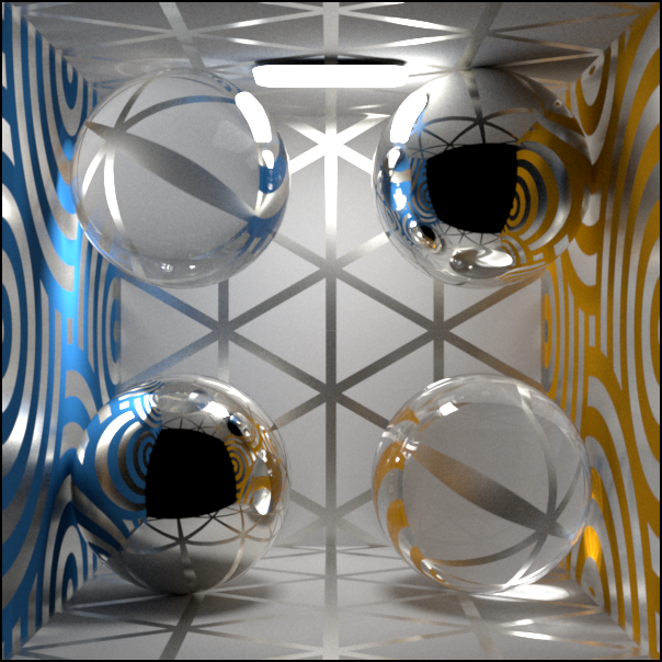
Spectral rendering mode#

Spectral + Polarized rendering mode#

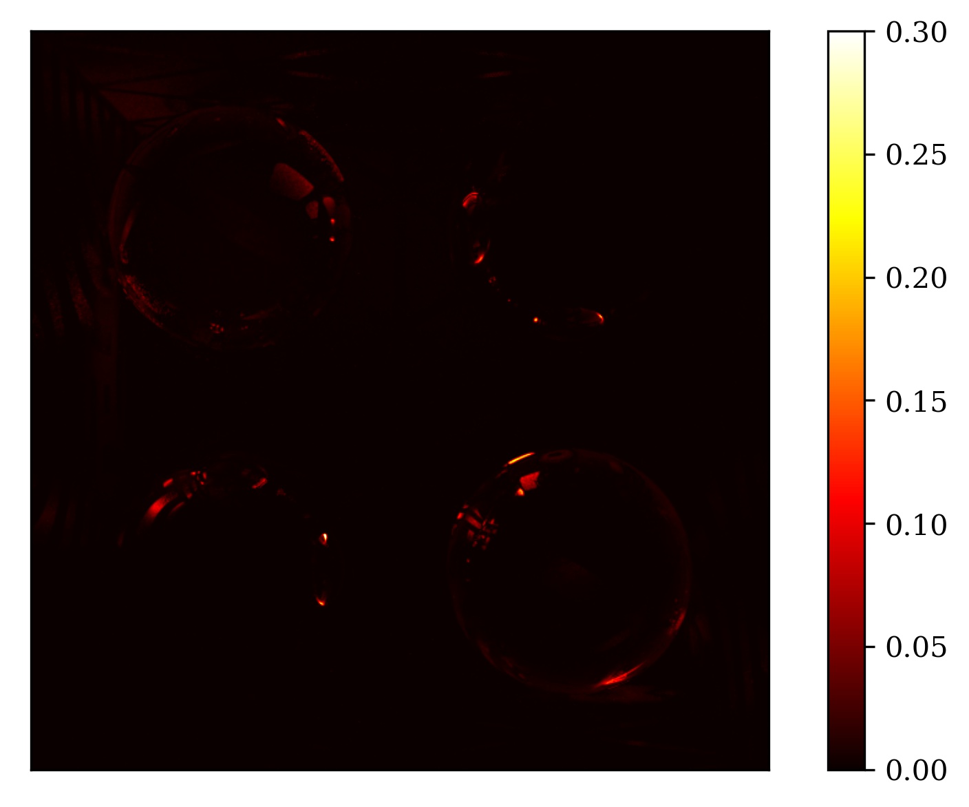
Pixel-wise absolute error between the two previous images.#

Alternatively, the difference is clearer when opening both images in separate tabs and switching between them.

Another simple but effective way to make the effects visible is to place a (rotating) linear polarizer in front of the camera. Such animations clearly show the underlying complexity that arises from accounting for polarization:

Stokes vector output

Mitsuba 3 can optionally also output the complete Stokes vector output at the end of the simulation by writing a multichannel EXR image. This is accomplished by switching to a special Stokes integrator plugin when setting up the scene description .xml file:

<integrator type="stokes">
    <!-- Note how there is still a normal path tracer nested inside that
         will do the actual simulation. -->
    <integrator type="path"/>
</integrator>

The output EXR images produced by this encodes the Stokes vectors with 16 channels in total:

• (0-3): The normal color (RGB) + alpha (A) channels.

• (4-6): \(\mathbf{s}_0\) (intensity) as an RGB image.

• (7-9): \(\mathbf{s}_1\) (horizontal vs. vertical polarization) as an RGB image.

• (10-12): \(\mathbf{s}_2\) (diagonal linear polarization) as an RGB image.

• (13-15): \(\mathbf{s}_3\) (right vs. left circular polarization) as an RGB image.

Currently, the Stokes components (\(\mathbf{s}_0, \dots, \mathbf{s}_3\)) will all go through the usual color conversion process at the end. In spectral mode, this can be problematic as Stokes vectors for different wavelengths will be integrated against XYZ sensitivity curves and finally converted to RGB colors (while still being signed quantities). This is likely not ideal for all applications, so alternatively we suggest to render images at fixed wavelengths. This can be achieved for instance by constructing scenes carefully s.t. only uniform spectra are used everywhere. Monochromatic or RGB rendering modes can be a useful tool here as these use “raw” floating point inputs and outputs. In comparison, spectral modes use an upsampling step to determine plausible spectra based on input RGB values which might not work as expected.

Internally, the Stokes integrator has to perform a last coordinate frame rotation to make sure the Stokes vector is saved in a consistent format, where its reference basis is aligned with the horizontal axis of the camera frame:

Or in source code:

The final alignment with the computed Stokes vector and the horizontal axis of the camera.

// From `src/integrators/stokes.cpp`

// Call a nested integrator (e.g. the path tracer)
auto [result, mask] = integrator->sample(scene, sampler, ray, ...);

// Compute the implicit Stokes reference for the incoming light path
Vector3f basis_out = mueller::stokes_basis(-ray.d);

// Get the camera transformation and evaluate for the current sampled `time`
Transform4f transform = scene->sensors()[0]->world_transform()->eval(ray.time);

// Compute the output Stokes reference that aligns horizontally with the camera
Vector3f vertical = transform * Vector3f(0.f, 1.f, 0.f);
Vector3f basis_cam = dr::cross(ray.d, vertical);

// Perform the final Mueller matrix reference frame rotation on the output
result = mueller::rotate_stokes_basis(-ray.d, basis_out, basis_cam) * result;

// Extract the first column of the Mueller matrix, i.e. the Stokes vector
auto const &stokes = result.entry(0);

Polarization visualizations

Mitsuba 3 also includes a separate command line tool to create commonly used visualizations from the EXR images with Stokes vector information, which can be run via Python, e.g.:

python -m mitsuba.python.polvis <filename>.exr <flags>

For instance, it can create the following false-color visualizations (green: positive, red: negative) of the Stokes components of the scene above:

\(\mathbf{s}_0\)#

\(\mathbf{s}_1\)#

\(\mathbf{s}_2\)#

\(\mathbf{s}_3\)#

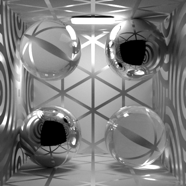
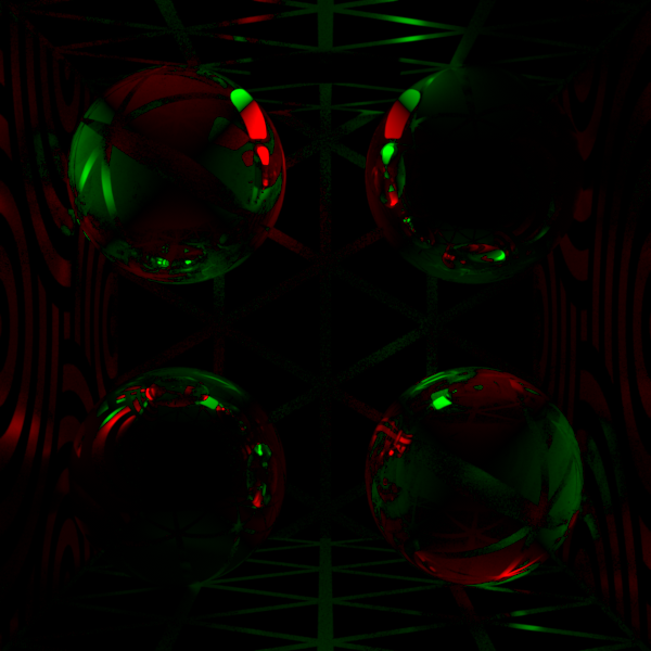
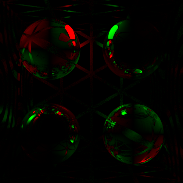
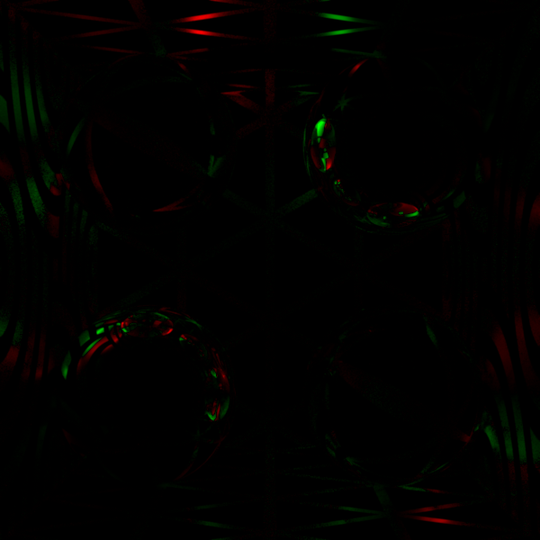
Alternatives that are more intuitive, originally proposed by Wilkie and Weidlich [WW10], are also supported. Please refer to the corresponding article for more information on these.

Degree of polarization#

Type of polarization (linear vs. circular)#

Orientation of linear polarization#

Chirality of circular polarization (left vs. right)#

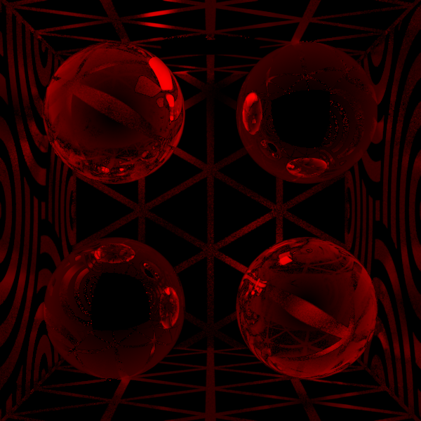
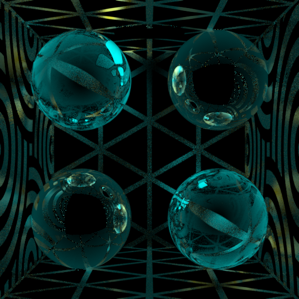
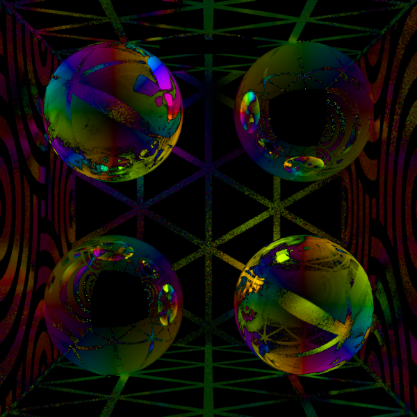
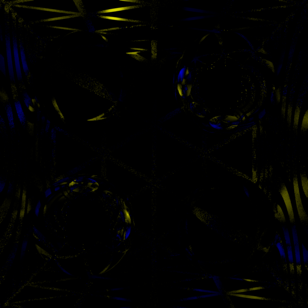
Choosing an integrator

Like for regular rendering, the normal path tracer is a great default choice for polarized rendering. But it does have one notable limitation that tends to come up in polarized scenes, especially ones that use optical elements (e.g. polarizers, retarders) for instance when using Mitsuba 3 to build a virtual version of optical experiments.

Consider the following (seemingly) simple Cornell box scene, where a relatively small light source is behind a linear polarizer:

In such scenes, a path tracer will normally rely heavily on the ability to connect shadow rays directly to the light source to account for the incoming illumination at a shading point. Unfortunately, the path tracer implemented in Mitsuba 3 is not able to do so through the linear polarizer and as a consequence, it has to rely on hitting the light source purely by chance after diffuse scattering on one of the walls. Depending on the size of the light source, this can be a source of very high variance that will take a long time to converge, see the image below (left).

Because light travels through the polarizer in a straight line (unlike for instance when rendering caustics through some glass objects), these shadow rays can in principle be traced through the filter. In such scenarios, it is recommended to switch to the volumetric path tracer that does have support for this (see image below, right) even if the scene does not actually contain any volumes.

Both of these images were rendered in roughly equal time at the same number of samples per pixel. The only difference is the choice of the integrator. Note also that both images are correct in expectation, and the path tracer will just need a much longer time to converge to the solution.

Rendered with the path tracer#

Rendered with the volumetric path tracer#

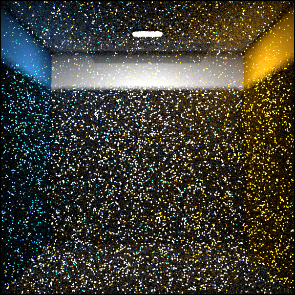
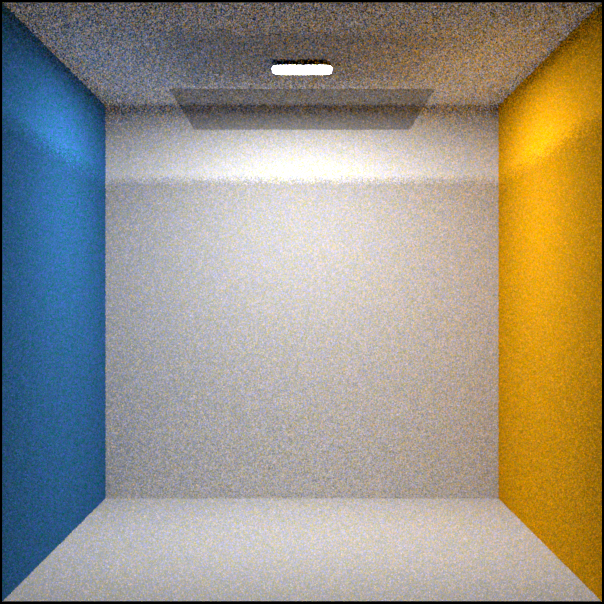
Feature list

The following plugins in Mitsuba 3 currently work/interact with polarization:

Integrators

• Direct illumination (direct)

• Path tracer (path)

• Volumetric path tracer when used for surfaces (volpath)

• Stokes integrator to extract polarization specific information (stokes)

BSDFs

• Smooth conductor (conductor)

• Smooth dielectric (dielectric)

• Rough conductor (roughconductor)

• Linear polarizer (polarizer)

• Linear retarder (retarder)

• Circular polarizer (circular)

• Null (null)

• Polarized plastic from [BJTK18] (pplastic)

• Measured polarized to render pBRDFs measured as part of [BZK+20] (measured_polarized)

Polarized BSDFs can also be combined or modified with these plugins:

• Blended material (blendbsdf)

• Bump map adapter (bumpmap)

• Normal map adapter (normalmap)

• Opacity mask (mask)

• Two-sided adapter (twosided)

All remaining BSDFs currently act as depolarizers.

---

At this point, the polarization support in Mitsuba 3 has two main functionalities that are missing: polarized emission and volumetric scattering.

Polarized emission

All emitters in Mitsuba 3 currently emit completely unpolarized light. This can be partially sidestepped for now by placing filters (e.g. linear polarizer) into the scene. A more complete solution would require careful Stokes reference basis conversions between emitter coordinate systems and world space, similarly as for the BSDF case (Section pBSDF evaluation and sampling).

Polarized volumetric scattering

While the volumetric path tracer (volpath) does support polarization when restricted to the surface case, it does not support polarized volumes. In particular, all phase functions in Mitsuba 3 act as depolarizers currently. Support for this would likely require small adjustments to the integrator (for tracking coordinate systems) and implementing some polarized phase function. A lot of the coordinate conversions from the BSDF case could probably be omitted as phase functions do not have a concept of local space and always operate in world space (Section pBSDF evaluation and sampling).