Integrators
In Mitsuba 3, the different rendering techniques are collectively referred to as integrators, since they perform integration over a high-dimensional space. Each integrator represents a specific approach for solving the light transport equation—usually favored in certain scenarios, but at the same time affected by its own set of intrinsic limitations. Therefore, it is important to carefully select an integrator based on user-specified accuracy requirements and properties of the scene to be rendered.
In the XML description language, a single integrator is usually instantiated by declaring it at the top level within the scene, e.g.
<scene version="3.0.0">
    <!-- Instantiate a unidirectional path tracer,
        which renders paths up to a depth of 5 -->
    <integrator type="path">
        <integer name="max_depth" value="5"/>
    </integrator>

    <!-- Some geometry to be rendered -->
    <shape type="sphere">
        <bsdf type="diffuse"/>
    </shape>
</scene>
'type': 'scene',
# Instantiate a unidirectional path tracer, which renders
# paths up to a depth of 5
'integrator_id': {
    'type': 'path',
    'max_depth': 5
},

# Some geometry to be rendered
'shape_id': {
    'type': 'sphere',
    'bsdf': {
        'type': 'diffuse'
    }
}
This section gives an overview of the available choices along with their parameters.
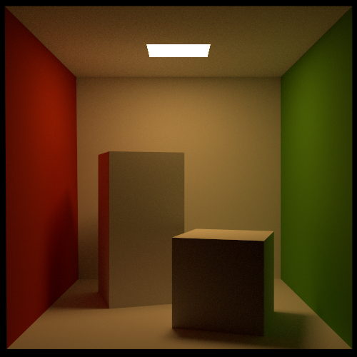
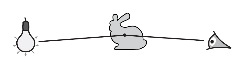
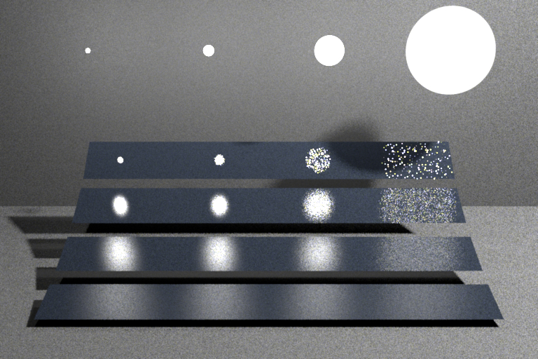
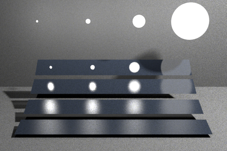
Almost all integrators use the concept of path depth. Here, a path refers to a chain of scattering events that starts at the light source and ends at the camera. It is often useful to limit the path depth when rendering scenes for preview purposes, since this reduces the amount of computation that is necessary per pixel. Furthermore, such renderings usually converge faster and therefore need fewer samples per pixel. When reference-quality is desired, one should always leave the path depth unlimited.
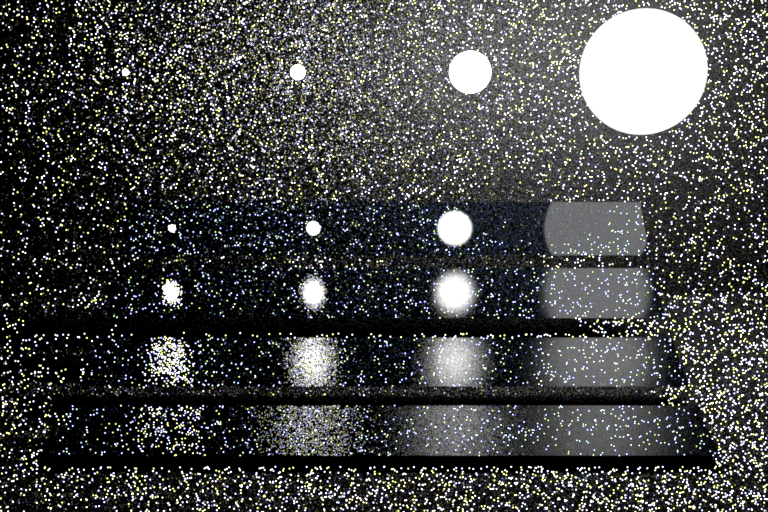
The Cornell box renderings below demonstrate the visual effect of a maximum path depth. As the paths are allowed to grow longer, the color saturation increases due to multiple scattering interactions with the colored surfaces. At the same time, the computation time increases.
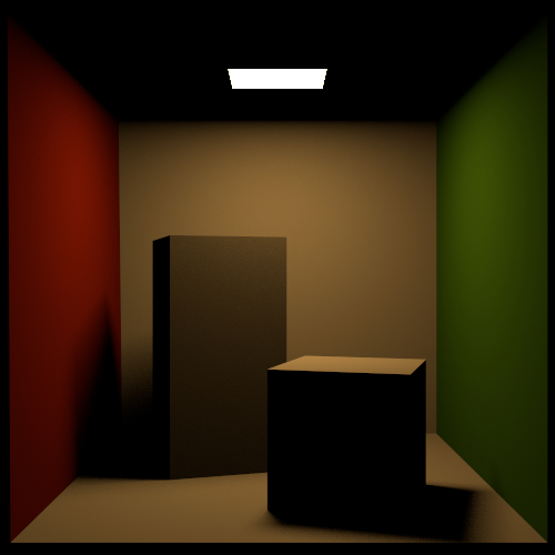
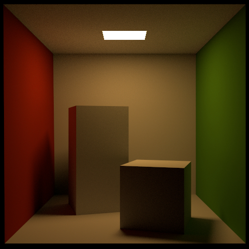
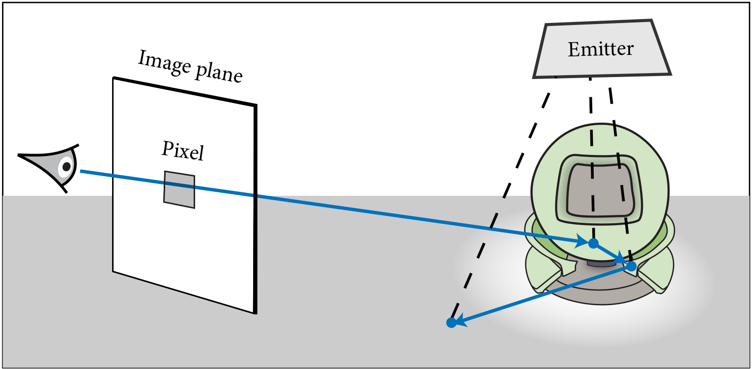
Mitsuba counts depths starting at 1, which corresponds to visible light sources (i.e. a path that starts at the light source and ends at the camera without any scattering interaction in between). A depth-2 path (also known as “direct illumination”) includes a single scattering event like shown here:
Direct illumination integrator (direct)
Parameter |
Type |
Description |
Flags |
|---|---|---|---|
shading_samples |
integer |
This convenience parameter can be used to set both |
|
emitter_samples |
integer |
Optional more fine-grained parameter: specifies the number of samples that should be generated using the direct illumination strategies implemented by the scene’s emitters. (Default: set to the value of shading_samples) |
|
bsdf_samples |
integer |
Optional more fine-grained parameter: specifies the number of samples that should be generated using the BSDF sampling strategies implemented by the scene’s surfaces. (Default: set to the value of shading_samples) |
|
hide_emitters |
boolean |
Hide directly visible emitters. (Default: no, i.e. false) |
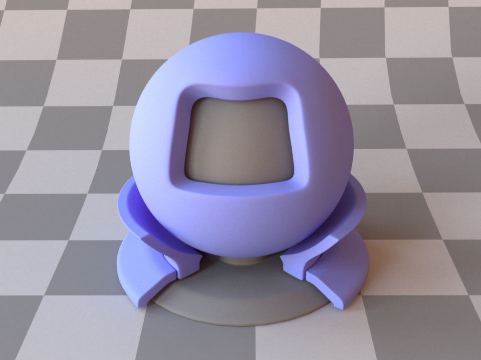
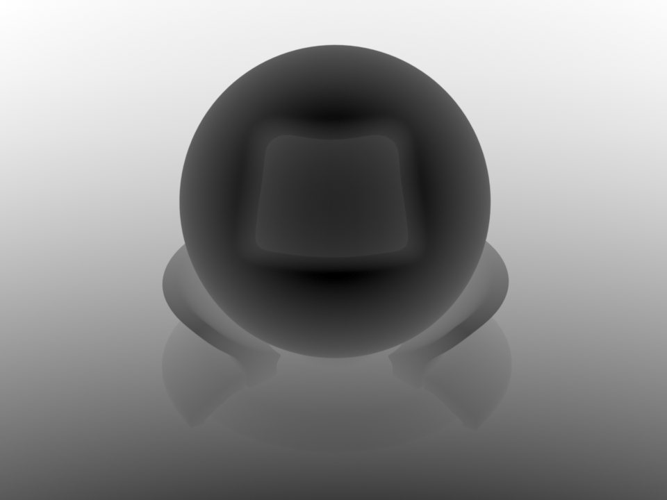
This integrator implements a direct illumination technique that makes use of multiple importance sampling: for each pixel sample, the integrator generates a user-specifiable number of BSDF and emitter samples and combines them using the power heuristic. Usually, the BSDF sampling technique works very well on glossy objects but does badly everywhere else (a), while the opposite is true for the emitter sampling technique (b). By combining these approaches, one can obtain a rendering technique that works well in both cases (c).
The number of samples spent on either technique is configurable, hence it is also possible to turn this plugin into an emitter sampling-only or BSDF sampling-only integrator.
Note
This integrator does not handle participating media or indirect illumination.
<integrator type="direct"/>
'type': 'direct'
Path tracer (path)
Parameter |
Type |
Description |
Flags |
|---|---|---|---|
max_depth |
integer |
Specifies the longest path depth in the generated output image (where -1 corresponds to \(\infty\)). A value of 1 will only render directly visible light sources. 2 will lead to single-bounce (direct-only) illumination, and so on. (Default: -1) |
|
rr_depth |
integer |
Specifies the path depth, at which the implementation will begin to use the russian roulette path termination criterion. For example, if set to 1, then path generation may randomly cease after encountering directly visible surfaces. (Default: 5) |
|
hide_emitters |
boolean |
Hide directly visible emitters. (Default: no, i.e. false) |
This integrator implements a basic path tracer and is a good default choice when there is no strong reason to prefer another method.
To use the path tracer appropriately, it is instructive to know roughly how it works: its main operation is to trace many light paths using random walks starting from the sensor. A single random walk is shown below, which entails casting a ray associated with a pixel in the output image and searching for the first visible intersection. A new direction is then chosen at the intersection, and the ray-casting step repeats over and over again (until one of several stopping criteria applies).
At every intersection, the path tracer tries to create a connection to the light source in an attempt to find a complete path along which light can flow from the emitter to the sensor. This of course only works when there is no occluding object between the intersection and the emitter.
This directly translates into a category of scenes where a path tracer can be expected to produce reasonable results: this is the case when the emitters are easily “accessible” by the contents of the scene. For instance, an interior scene that is lit by an area light will be considerably harder to render when this area light is inside a glass enclosure (which effectively counts as an occluder).
Like the direct plugin, the path tracer internally relies on multiple importance sampling to combine BSDF and emitter samples. The main difference in comparison to the former plugin is that it considers light paths of arbitrary length to compute both direct and indirect illumination.
Note
This integrator does not handle participating media
<integrator type="path">
    <integer name="max_depth" value="8"/>
</integrator>
'type': 'path',
'max_depth': 8
Arbitrary Output Variables integrator (aov)
Parameter |
Type |
Description |
Flags |
|---|---|---|---|
aovs |
string |
List of <name>:<type> pairs denoting the enabled AOVs. |
|
(Nested plugin) |
integrator |
Sub-integrators (can have more than one) which will be sampled along the AOV integrator. Their respective output will be put into distinct images. |
This integrator returns one or more AOVs (Arbitrary Output Variables) describing the visible surfaces.
Here is an example on how to enable the depth and shading normal AOVs while still rendering the
image with a path tracer. The RGBA image produces by the path tracer will be stored in the
[my_image.R, my_image.G, my_image.B, my_image.A] channels of the EXR
output file.
<integrator type="aov">
    <string name="aovs" value="dd.y:depth,nn:sh_normal"/>
    <integrator type="path" name="my_image"/>
</integrator>
'type': 'aov',
'aovs': 'dd.y:depth,nn:sh_normal',
'my_image': {
    'type': 'path',
}
Currently, the following AOVs types are available:
albedo: Albedo (diffuse reflectance) of the material.
depth: Distance from the pinhole.
position: World space position value.
uv: UV coordinates.
geo_normal: Geometric normal.
sh_normal: Shading normal.
dp_du, dp_dv: Position partials wrt. the UV parameterization.
duv_dx, duv_dy: UV partials wrt. changes in screen-space.
prim_index: Primitive index (e.g. triangle index in the mesh).
shape_index: Shape index.
Note that integer-valued AOVs (e.g. prim_index, shape_index) are meaningless whenever there is only partial pixel coverage or when using a wide pixel reconstruction filter as it will result in fractional values.
The albedo AOV will evaluate the diffuse reflectance (ref BSDF::eval_diffuse_reflectance) of the material. Note that depending on the material, this value might only be an approximation.
Volumetric path tracer (volpath)
Parameter |
Type |
Description |
Flags |
|---|---|---|---|
max_depth |
integer |
Specifies the longest path depth in the generated output image (where -1 corresponds to \(\infty\)). A value of 1 will only render directly visible light sources. 2 will lead to single-bounce (direct-only) illumination, and so on. (Default: -1) |
|
rr_depth |
integer |
Specifies the minimum path depth, after which the implementation will start to use the russian roulette path termination criterion. (Default: 5) |
|
hide_emitters |
boolean |
Hide directly visible emitters. (Default: no, i.e. false) |
This plugin provides a volumetric path tracer that can be used to compute approximate solutions of the radiative transfer equation. Its implementation makes use of multiple importance sampling to combine BSDF and phase function sampling with direct illumination sampling strategies. On surfaces, it behaves exactly like the standard path tracer.
This integrator has special support for index-matched transmission events (i.e. surface scattering events that do not change the direction of light). As a consequence, participating media enclosed by a stencil shape are rendered considerably more efficiently when this shape has a null or thin dielectric BSDF assigned to it (as compared to, say, a dielectric or roughdielectric BSDF).
Note
This integrator does not implement good sampling strategies to render participating media with a spectrally varying extinction coefficient. For these cases, it is better to use the more advanced volumetric path tracer with spectral MIS, which will produce in a significantly less noisy rendered image.
Warning
This integrator does not support forward-mode differentiation.
<integrator type="volpath">
    <integer name="max_depth" value="8"/>
</integrator>
'type': 'volpath',
'max_depth': 8
Volumetric path tracer with spectral MIS (volpathmis)
Parameter |
Type |
Description |
Flags |
|---|---|---|---|
max_depth |
integer |
Specifies the longest path depth in the generated output image (where -1 corresponds to \(\infty\)). A value of 1 will only render directly visible light sources. 2 will lead to single-bounce (direct-only) illumination, and so on. (Default: -1) |
|
rr_depth |
integer |
Specifies the minimum path depth, after which the implementation will start to use the russian roulette path termination criterion. (Default: 5) |
|
hide_emitters |
boolean |
Hide directly visible emitters. (Default: no, i.e. false) |
This plugin provides a volumetric path tracer that can be used to compute approximate solutions of the radiative transfer equation. Its implementation performs MIS both for directional sampling as well as free-flight distance sampling. In particular, this integrator is well suited to render media with a spectrally varying extinction coefficient. The implementation is based on the method proposed by Miller et al. [MGJ19] and is only marginally slower than the simple volumetric path tracer.
Similar to the simple volumetric path tracer, this integrator has special support for index-matched transmission events.
Warning
This integrator does not support forward-mode differentiation.
<integrator type="volpathmis">
    <integer name="max_depth" value="8"/>
</integrator>
'type': 'volpathmis',
'max_depth': 8
Path Replay Backpropagation (prb)
Parameter |
Type |
Description |
Flags |
|---|---|---|---|
max_depth |
integer |
Specifies the longest path depth in the generated output image (where -1 corresponds to \(\infty\)). A value of 1 will only render directly visible light sources. 2 will lead to single-bounce (direct-only) illumination, and so on. (Default: 6) |
|
rr_depth |
integer |
Specifies the path depth, at which the implementation will begin to use the russian roulette path termination criterion. For example, if set to 1, then path generation many randomly cease after encountering directly visible surfaces. (Default: 5) |
|
hide_emitters |
boolean |
Hide directly visible emitters. (Default: no, i.e. false) |
This plugin implements a basic Path Replay Backpropagation (PRB) integrator with the following properties:
Emitter sampling (a.k.a. next event estimation).
Russian Roulette stopping criterion.
No projective sampling. This means that the integrator cannot be used for shape optimization (it will return incorrect/biased gradients for geometric parameters like vertex positions.)
Detached sampling. This means that the properties of ideal specular objects (e.g., the IOR of a glass vase) cannot be optimized.
See prb_basic.py for an even more reduced implementation that removes
the first two features.
See the papers [VSJ21] and [ZSGJ21] for details on PRB, attached/detached sampling.
Warning
This integrator is not supported in variants which track polarization states.
'type': 'prb',
'max_depth': 8
Basic Path Replay Backpropagation (prb_basic)
Parameter |
Type |
Description |
Flags |
|---|---|---|---|
max_depth |
integer |
Specifies the longest path depth in the generated output image (where -1 corresponds to \(\infty\)). A value of 1 will only render directly visible light sources. 2 will lead to single-bounce (direct-only) illumination, and so on. (Default: 6) |
|
hide_emitters |
boolean |
Hide directly visible emitters. (Default: no, i.e. false) |
Basic Path Replay Backpropagation-style integrator without next event estimation, multiple importance sampling, Russian Roulette, and projective sampling. The lack of all of these features means that gradients are noisy and don’t correctly account for visibility discontinuities. The lack of a Russian Roulette stopping criterion means that generated light paths may be unnecessarily long and costly to generate.
This class is not meant to be used in practice, but merely exists to
illustrate how a very basic rendering algorithm can be implemented in
Python along with efficient forward/reverse-mode derivatives. See the file
prb.py for a more feature-complete Path Replay Backpropagation
integrator, and prb_reparam.py for one that also handles visibility.
Warning
This integrator is not supported in variants which track polarization states.
'type': 'prb_basic',
'max_depth': 8
Direct illumination projective sampling (direct_projective)
Parameter |
Type |
Description |
Flags |
|---|---|---|---|
sppc |
integer |
Number of samples per pixel used to estimate the continuous
derivatives. Unless it is zero, this parameter is overriden by the
|
|
sppp |
integer |
Number of samples per pixel used to to estimate the gradients resulting
from primary visibility changes (on the first segment of the light
path: from the sensor to the first bounce) derivatives. Unless it is
zero, this parameter is overriden by the |
|
sppi |
integer |
Number of samples per pixel used to to estimate the gradients resulting
from indirect visibility changes derivatives. Unless it is zero, this
parameter is overriden by the |
|
guiding |
string |
Guiding type, must be one of: “none”, “grid”, or “octree”. This specifies the guiding method used for indirectly observed discontinuities. (Default: “octree”) |
|
guiding_proj |
boolean |
Whether or not to use projective sampling to generate the set of samples that are used to build the guiding structure. (Default: True) |
|
guiding_rounds |
integer |
Number of sampling iterations used to build the guiding data structure. A higher number of rounds will use more samples and hence should result in a more accurate guiding structure. (Default: 1) |
This plugin implements a projective sampling direct illumination integrator with the following features:
Emitter sampling (a.k.a. next event estimation).
Projective sampling. This means that it can handle discontinuous visibility changes, such as a moving shape’s gradients.
Detached sampling. This means that the properties of ideal specular objects (e.g., the IOR of a glass vase) cannot be optimized.
See the paper [ZRJ23] for details on projective sampling, and guiding structures for indirect visibility discontinuities.
It is functionally equivalent with prb_projective when max_depth is set
to be 2.
Warning
This integrator is not supported in variants which track polarization states.
'type': 'direct_projective',
'sppc': 32,
'sppp': 32,
'sppi': 128,
'guiding': 'octree',
'guiding_proj': True,
'guiding_rounds': 1
Projective sampling Path Replay Backpropagation (PRB) (prb_projective)
Parameter |
Type |
Description |
Flags |
|---|---|---|---|
max_depth |
integer |
Specifies the longest path depth in the generated output image (where -1 corresponds to \(\infty\)). A value of 1 will only render directly visible light sources. 2 will lead to single-bounce (direct-only) illumination, and so on. (Default: -1) |
|
rr_depth |
integer |
Specifies the path depth, at which the implementation will begin to use the russian roulette path termination criterion. For example, if set to 1, then path generation many randomly cease after encountering directly visible surfaces. (Default: 5) |
|
sppc |
integer |
Number of samples per pixel used to estimate the continuous
derivatives. Unless it is zero, this parameter is overriden by the
|
|
sppp |
integer |
Number of samples per pixel used to to estimate the gradients resulting
from primary visibility changes (on the first segment of the light
path: from the sensor to the first bounce) derivatives. Unless it is
zero, this parameter is overriden by the |
|
sppi |
integer |
Number of samples per pixel used to to estimate the gradients resulting
from indirect visibility changes derivatives. Unless it is zero, this
parameter is overriden by the |
|
guiding |
string |
Guiding type, must be one of: “none”, “grid”, or “octree”. This specifies the guiding method used for indirectly observed discontinuities. (Default: “octree”) |
|
guiding_proj |
boolean |
Whether or not to use projective sampling to generate the set of samples that are used to build the guiding structure. (Default: True) |
|
guiding_rounds |
integer |
Number of sampling iterations used to build the guiding data structure. A higher number of rounds will use more samples and hence should result in a more accurate guiding structure. (Default: 1) |
This plugin implements a projective sampling Path Replay Backpropagation (PRB) integrator with the following features:
Emitter sampling (a.k.a. next event estimation).
Russian Roulette stopping criterion.
Projective sampling. This means that it can handle discontinuous visibility changes, such as a moving shape’s gradients.
Detached sampling. This means that the properties of ideal specular objects (e.g., the IOR of a glass vase) cannot be optimized.
In order to estimate the indirect visibility discontinuous derivatives, this
integrator starts by sampling a boundary segment and then attempts to
connect it to the sensor and an emitter. It is effectively building lights
paths from the middle outwards. In order to stay within the specified
max_depth, the integrator starts by sampling a path to the sensor by using
reservoir sampling to decide whether or not to use a longer path. Once a
path to the sensor is found, the other half of the full light path is
sampled.
See the paper [ZRJ23] for details on projective sampling, and guiding structures for indirect visibility discontinuities.
Warning
This integrator is not supported in variants which track polarization states.
'type': 'prb_projective',
'sppc': 32,
'sppp': 32,
'sppi': 128,
'guiding': 'octree',
'guiding_proj': True,
'guiding_rounds': 1
Path Replay Backpropagation Volumetric Integrator (prbvolpath)
Parameter |
Type |
Description |
Flags |
|---|---|---|---|
max_depth |
integer |
Specifies the longest path depth in the generated output image (where -1 corresponds to \(\infty\)). A value of 1 will only render directly visible light sources. 2 will lead to single-bounce (direct-only) illumination, and so on. (Default: 6) |
|
rr_depth |
integer |
Specifies the path depth, at which the implementation will begin to use the russian roulette path termination criterion. For example, if set to 1, then path generation many randomly cease after encountering directly visible surfaces. (Default: 5) |
|
hide_emitters |
boolean |
Hide directly visible emitters. (Default: no, i.e. false) |
This class implements a volumetric Path Replay Backpropagation (PRB) integrator with the following properties:
Differentiable delta tracking for free-flight distance sampling
Emitter sampling (a.k.a. next event estimation).
Russian Roulette stopping criterion.
No projective sampling. This means that the integrator cannot be used for shape optimization (it will return incorrect/biased gradients for geometric parameters like vertex positions.)
Detached sampling. This means that the properties of ideal specular objects (e.g., the IOR of a glass vase) cannot be optimized.
See the paper [VSJ21] for details on PRB and differentiable delta tracking.
Warning
This integrator is not supported in variants which track polarization states.
'type': 'prbvolpath',
'max_depth': 8
Depth integrator (depth)
Example of one an extremely simple type of integrator that is also helpful for debugging: returns the distance from the camera to the closest intersected object, or 0 if no intersection was found.
<integrator type="depth"/>
'type': 'depth'
Moment integrator (moment)
Parameter |
Type |
Description |
Flags |
|---|---|---|---|
(Nested plugin) |
integrator |
Sub-integrators (can have more than one) which will be sampled along the AOV integrator. Their respective XYZ output will be put into distinct images. |
This integrator returns one AOVs recording the second moment of the samples of the nested integrator.
<integrator type="moment">
    <integrator type="path"/>
</integrator>
'type': 'moment',
'nested': {
    'type': 'path',
}
Stokes vector integrator (stokes)
Parameter |
Type |
Description |
Flags |
|---|---|---|---|
(Nested plugin) |
integrator |
Sub-integrator (only one can be specified) which will be sampled along the Stokes integrator. In polarized rendering modes, its output Stokes vector is written into distinct images. |
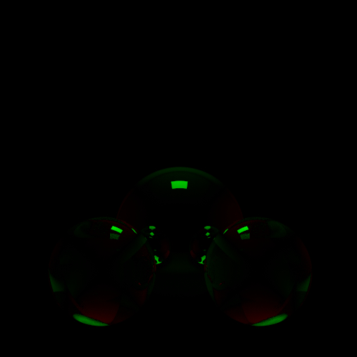
This integrator returns a multi-channel image describing the complete measured polarization state at the sensor, represented as a Stokes vector \(\mathbf{s}\).
Here we show an example monochrome output in a scene with two dielectric and one conductive sphere that all affect the polarization state of the (initially unpolarized) light.
The first entry corresponds to usual radiance, whereas the remaining three entries describe the polarization of light shown as false color images (green: positive, red: negative).
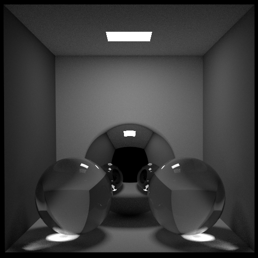
“\(\mathbf{s}_0\)”: radiance
“\(\mathbf{s}_1\)”: horizontal vs. vertical polarization
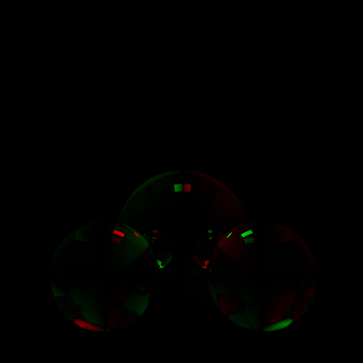
“\(\mathbf{s}_2\)”: positive vs. negative diagonal polarization
“\(\mathbf{s}_3\)”: right vs. left circular polarization
In the following example, a normal path tracer is nested inside the Stokes vector integrator:
<integrator type="stokes">
    <integrator type="path">
        <!-- path tracer parameters -->
    </integrator>
</integrator>
'type': 'stokes',
'nested': {
    'type': 'path',
    # .. path tracer parameters
}
Particle tracer (ptracer)
Parameter |
Type |
Description |
Flags |
|---|---|---|---|
max_depth |
integer |
Specifies the longest path depth in the generated output image (where -1 corresponds to \(\infty\)). A value of 1 will only render directly visible light sources. 2 will lead to single-bounce (direct-only) illumination, and so on. (Default: -1) |
|
rr_depth |
integer |
Specifies the minimum path depth, after which the implementation will start to use the russian roulette path termination criterion. (Default: 5) |
|
hide_emitters |
boolean |
Hide directly visible emitters. (Default: no, i.e. false) |
|
samples_per_pass |
boolean |
If specified, divides the workload in successive passes with samples_per_pass samples per pixel. |
This integrator traces rays starting from light sources and attempts to connect them to the sensor at each bounce. It does not support media (volumes).
Usually, this is a relatively useless rendering technique due to its high variance, but there are some cases where it excels. In particular, it does a good job on scenes where most scattering events are directly visible to the camera.
Note that unlike sensor-based integrators such as path, it is not possible to divide the workload in image-space tiles. The samples_per_pass parameter allows splitting work in successive passes of the given sample count per pixel. It is particularly useful in wavefront mode.
<integrator type="ptracer">
    <integer name="max_depth" value="8"/>
</integrator>
'type': 'ptracer',
'max_depth': 8