Mesh I/O and manipulation
Reading a mesh from disk
Mitsuba provides an abstract Shape class to handle all geometric shapes. For triangle meshes, it has a concrete class Mesh that is further extended by 3 plugins which can load meshes directly from a file:
OBJ: handles meshes containing triangles and quadrilaterals from Wavefront OBJ files
PLY: handles Stanford PLY format meshes (both the ASCII and binary format)
Serialized: Mitsuba 0.6 serialized mesh format.
As any other Mitsuba object, we can use the load_dict function to instantiate one of these three plugins. They each have their own specific input parameters which you’ll find in their respective documentation, but here are the input parameters they all share:
filename: filename of the mesh file that should be loaded
face_normals: when set to true, any existing or computed vertex normals are discarded and face normals will instead be used during rendering. This gives the rendered object a faceted appearance.
to_world: specifies an linear object-to-world transformation.
Let’s now load a mesh and start playing with it.
[2]:
bunny = mi.load_dict({
    "type": "ply",
    "filename": "../scenes/meshes/bunny.ply",
    "face_normals": False,
    "to_world": mi.ScalarTransform4f().rotate([0, 0, 1], angle=10),
})

print(bunny)
PLYMesh[
  name = "bunny.ply",
  bbox = BoundingBox3f[
    min = [-0.0779344, -0.0611472, -0.0738726],
    max = [0.0874787, 0.0992267, 0.0468007]
  ],
  vertex_count = 35947,
  vertices = [843 KiB of vertex data],
  face_count = 69451,
  faces = [814 KiB of face data],
  face_normals = 0
]
The string representation of a Mesh object gives an overview of its size. If you wish to access some of these values, they are available through the following methods Shape.bbox(), Mesh.vertex_count(), Mesh.face_count().
Procedural mesh
By directly using the Mesh class, it is also possible to procedurally create a mesh. To illustrate this, we will build a spanning triangle disk and give it a wavy fringe. The exact details of how the vertex positions and face indices are generated are not important for the purposes of this guide. However, we do leave them as comments in the code.
[3]:
# Wavy disk construction
#
# Let N define the total number of vertices, the first N-1 vertices will compose
# the fringe of the disk, while the last vertex should be placed at the center.
# The first N-1 vertices must have their height modified such that they oscillate
# with some given frequency and amplitude. To compute the face indices, we define
# the first vertex of every face to be the vertex at the center (idx=N-1) and the
# other two can be assigned sequentially (modulo N-2).

# Disk with a wavy fringe parameters
N = 100
frequency = 12.0
amplitude = 0.4

# Generate the vertex positions
theta = dr.linspace(mi.Float, 0.0, dr.two_pi, N)
x, y = dr.sincos(theta)
z = amplitude * dr.sin(theta * frequency)
vertex_pos = mi.Point3f(x, y, z)

# Move the last vertex to the center
vertex_pos[dr.arange(mi.UInt32, N) == N - 1] = 0.0

# Generate the face indices
idx = dr.arange(mi.UInt32, N - 1)
face_indices = mi.Vector3u(N - 1, (idx + 1) % (N - 2), idx % (N - 2))
The Mesh constructor allocates all the necessary buffers to hold its data. Specifically, the constructor takes as arguments the number of vertices and faces which will then be fixed. It is not possible to edit a mesh in a way that would require the buffers to be resized (more/less faces for examples), a new Mesh would need to be created for such use cases. The constructor can also takes two boolean arguments has_vertex_normals and has_vertex_texcoords that must also be know at
the construction of the object, in order to allocate the appropriate buffers.
[4]:
# Create an empty mesh (allocates buffers of the correct size)
mesh = mi.Mesh(
    "wavydisk",
    vertex_count=N,
    face_count=N - 1,
    has_vertex_normals=False,
    has_vertex_texcoords=False,
)
In order to assign our existing vertex positions and face indices to the newly created Mesh object we will use the traverse() mechanism. All of the allocated buffers of a Mesh object are exposed, and can therefore be modified with this mechanism. This approach has the advantage of simplifying some of the assignment operations. In addition, if any vertex position is modified, a call to SceneParameters.update() will trigger recomputation of both the bounding box and vertex normals.
One caveat here is that meshes in Mitsuba store their data in flat linear buffers. Hence it is necessary to change the layout of the array of vertex positions and face indices computed above. Luckily, Dr.Jit provides dr.ravel() which does exactly that. The complement of this function is dr.unravel() which will convert a flat linear array to a structure-of-array of the specific type (e.g., Point3f).
[5]:
mesh_params = mi.traverse(mesh)
mesh_params["vertex_positions"] = dr.ravel(vertex_pos)
mesh_params["faces"] = dr.ravel(face_indices)
print(mesh_params.update())
[(Mesh[
  name = "wavydisk",
  bbox = BoundingBox3f[
    min = [-0.999874, -0.999497, -0.399547],
    max = [0.999874, 1, 0.399547]
  ],
  vertex_count = 100,
  vertices = [1.17 KiB of vertex data],
  face_count = 99,
  faces = [1.16 KiB of face data],
  face_normals = 0
], {'vertex_positions', 'faces'})]
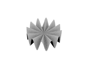
And now let’s take a look at our new mesh!
[6]:
scene = mi.load_dict({
    "type": "scene",
    "integrator": {"type": "path"},
    "light": {"type": "constant"},
    "sensor": {
        "type": "perspective",
        "to_world": mi.ScalarTransform4f().look_at(
            origin=[0, -5, 5], target=[0, 0, 0], up=[0, 0, 1]
        ),
    },
    "wavydisk": mesh,
})

img = mi.render(scene)

from matplotlib import pyplot as plt

plt.axis("off")
plt.imshow(mi.util.convert_to_bitmap(img));
Writing a mesh to disk
No matter how a Mesh object was loaded or built, it can always be exported to a PLY file format using the Mesh.write_ply() method. No other file formats are currently supported.
🗒 Note
Any mesh attribute (see below) that is attached to the object at the time when Mesh.write_ply() is called will be written to output file as a property. Mitsuba therefore allows you to create complex procedural properties for your meshes and export them to be used in some other context entirely.
[7]:
mesh.write_ply("wavydisk.ply")
Adding and editing attributes
Meshes in Mitsuba can have additional attributes per face or per vertex. Each attribute is either one or several floating point numbers, no other types are supported.
The Mesh.add_attribute() methods lets you define new attributes by giving them a name, a number of feilds, and their initial values. The attribute name must be prefixed with either vertex_ or face_, as this defines whether the attribute is defined for each face or for each vertex. For this example, we will be adding a RGB color to each vertex.
Moreover, Mitsuba 3 has a mesh attribute texture plugin that conviently allows you to visualize attributes.
[8]:
mesh = mi.load_dict({
    "type": "ply",
    "filename": "wavydisk.ply",
    "bsdf": {
        "type": "diffuse",
        "reflectance": {
            "type": "mesh_attribute",
            "name": "vertex_color",  # This will be used to visualize our attribute
        },
    },
})

# Needs to start with vertex_ or face_
attribute_size = mesh.vertex_count() * 3
mesh.add_attribute(
    "vertex_color", 3, [0] * attribute_size
)  # Add 3 floats per vertex (initialized at 0)
Once an attribute is created it can still be modified using the traverse() mechanism. As shown below, the attribute’s buffer will be exposed with a key corresponding to the attribute’s name.
[9]:
mesh_params = mi.traverse(mesh)
mesh_params
[9]:
SceneParameters[
  ---------------------------------------------------------------------------------
  Name                          Flags    Type  Parent
  ---------------------------------------------------------------------------------
  bsdf.reflectance.scale                 float MeshAttribute
  silhouette_sampling_weight             float PLYMesh
  faces                                  UInt  PLYMesh
  vertex_positions              ∂, D     Float PLYMesh
  vertex_normals                ∂, D     Float PLYMesh
  vertex_texcoords              ∂        Float PLYMesh
  vertex_color                  ∂        Float PLYMesh
]
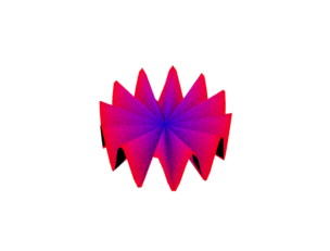
We can now easily change the values of the attribute using some simple Dr.Jit arithmetic.
[10]:
N = mesh.vertex_count()

vertex_colors = dr.zeros(mi.Float, 3 * N)
fringe_vertex_indices = dr.arange(mi.UInt, N - 1)
dr.scatter(vertex_colors, 1, fringe_vertex_indices * 3)  # Fringe is red
dr.scatter(vertex_colors, 1, [(N - 1) * 3 + 2])  # Center is blue

mesh_params["vertex_color"] = vertex_colors
mesh_params.update()
[10]:
[(PLYMesh[
    name = "wavydisk.ply",
    bbox = BoundingBox3f[
      min = [-0.999874, -0.999497, -0.399547],
      max = [0.999874, 1, 0.399547]
    ],
    vertex_count = 100,
    vertices = [3.52 KiB of vertex data],
    face_count = 99,
    faces = [1.16 KiB of face data],
    face_normals = 0,
    mesh attributes = [
      vertex_color: 3 floats
    ]
  ],
  {'vertex_color'})]
And visualize the result!
[11]:
scene = mi.load_dict(
    {
        "type": "scene",
        "integrator": {"type": "path"},
        "light": {"type": "constant"},
        "sensor": {
            "type": "perspective",
            "to_world": mi.ScalarTransform4f().look_at(
                origin=[0, -5, 5], target=[0, 0, 0], up=[0, 0, 1]
            ),
        },
        "wavydisk": mesh,
    }
)

img = mi.render(scene)

plt.axis("off")
plt.imshow(mi.util.convert_to_bitmap(img));