Rendering from multiple view points
Overview
In this tutorial, you will learn how to render a given scene from multiple points of view. This can be very convenient if you wish to generate a large synthetic dataset, or are doing some multi-view optimization.
🚀 You will learn how to:
Load Mitsuba objects
Create sensors
Render a scene from a specified sensor
Setup
Let us start by importing mitsuba and setting the variant.
[1]:
import mitsuba as mi
mi.set_variant("scalar_rgb")
Loading a scene
In previous tutorials, we have seen how to load a Mitsuba scene from an XML file. In Mitsuba 3, it is also possbile to load a scene defined by Python dictionary using load_dict().
In fact, the load_dict() function allows us to load any Mitsuba object by describing it as a Python dict. The exact form of the dictionary can be easily deduced from the equivalent XML representation, and more information on this subject can be found in the dedicated documentation chapter. The plugin
documentation also shows how to load each plugin using either XML or dict. Everything achievable with the XML scene format should be achievable using Python dicts as well.
In the following cell, we instantiate a scene containing a teapot mesh and a constant light source. This tutorial makes heavy use of the ScalarTransform4f class to create transformations. Take a look at the dedicated How-to Guide for more information on how to use it.
🗒 Note
Notice the Scalar prefix in ScalarTransform4f. This indicates that no matter which variant of Mitsuba is enabled, this type will always refer to the CPU scalar transformation type (which can also be accessed with mitsuba.scalar_rgb.Transform4f. The same applies to all basic types (e.g. Float, UInt32) and other data-structure type (e.g. Ray3f, SurfaceInteraction3f), which can all be prefixed with Scalar to obtain the corresponding CPU scalar type.
[2]:
# Create an alias for convenience
from mitsuba import ScalarTransform4f as T

scene = mi.load_dict({
    'type': 'scene',
    # The keys below correspond to object IDs and can be chosen arbitrarily
    'integrator': {'type': 'path'},
    'light': {'type': 'constant'},
    'teapot': {
        'type': 'ply',
        'filename': '../scenes/meshes/teapot.ply',
        'to_world': T().translate([0, 0, -1.5]),
        'bsdf': {
            'type': 'diffuse',
            'reflectance': {'type': 'rgb', 'value': [0.1, 0.2, 0.3]},
        },
    },
})
Next, let’s create our sensors!
Creating sensors
Mitsuba provides a high level Sensor abstraction, along with a Film abstraction, which define how radiance from our scene should be recorded. For the purpose of this tutorial, we will focus on the sensor’s placement and skip over all other parameters. Of course, if you wished to do so, it is entirely possible to define multiple radically different sensors. You can learn more about the different types of sensors and films that are included in Mitsuba in the plugin
documentation.
In this tutorial, we are going to render our scene from multiple points of view placed around the teapot in a circular fashion. To this end, let’s define a helper function load_sensor that creates a sensor with a specific position given as input in spherical coordinates. As previously mentionned, load_dict() can be used to load a single Mitsuba object too and not just entire scenes, so let’s make use of it here.
Note that although we create a new sampler and film per sensor instance, it is possible to create a single instance of each that are then shared by all sensors.
[3]:
def load_sensor(r, phi, theta):
    # Apply two rotations to convert from spherical coordinates to world 3D coordinates.
    origin = T().rotate([0, 0, 1], phi).rotate([0, 1, 0], theta) @ mi.ScalarPoint3f([0, 0, r])

    return mi.load_dict({
        'type': 'perspective',
        'fov': 39.3077,
        'to_world': T().look_at(
            origin=origin,
            target=[0, 0, 0],
            up=[0, 0, 1]
        ),
        'sampler': {
            'type': 'independent',
            'sample_count': 16
        },
        'film': {
            'type': 'hdrfilm',
            'width': 256,
            'height': 256,
            'rfilter': {
                'type': 'tent',
            },
            'pixel_format': 'rgb',
        },
    })
Rendering using a specific sensor
The render() function can take quite a few aditional arguments. In a previous tutorial, we have seen that we can specify the number of samples per pixel with the keyword argument spp. We can also dynamically specify a sensor with the sensor keyword argument that should be used instead of the first sensor defined in the scene, which would be used by default. The previous
tutorial showed how mi.traverse can be used to edit scenes. That same mechanism could be used to edit the sensor after each render. However, we would be limited to editing the parameters that are exposed by the object. The sensor keyword argument of render is therefore much more powerful if you wish to render a same scene from mulitple points of view.
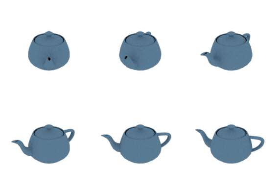
In this example, we place the sensors at a fixed latitude (defined by theta) on a large sphere of radius radius centered on the teapot, and vary the longitude with different values of \(\phi\) (defined by phis).
[4]:
sensor_count = 6

radius = 12
phis = [20.0 * i for i in range(sensor_count)]
theta = 60.0

sensors = [load_sensor(radius, phi, theta) for phi in phis]
We are now ready to render from each of our sensors.
[5]:
images = [mi.render(scene, spp=16, sensor=sensor) for sensor in sensors]
Finally, we can use the convenient Bitmap class to quickly visualize our six rendered images directly in the notebook.
[6]:
from matplotlib import pyplot as plt
fig = plt.figure(figsize=(10, 7))
fig.subplots_adjust(wspace=0, hspace=0)
for i in range(sensor_count):
    ax = fig.add_subplot(2, 3, i + 1).imshow(images[i] ** (1.0 / 2.2))
    plt.axis("off")