Mitsuba quickstart
Overview
In this tutorial, you will render your very first image using Mitsuba 3!
🚀 You will learn how to:
Import Mitsuba in Python and set the “variant”
Load a scene from disk
Render a scene
Write a rendered image to disk
Importing Mitsuba
After installing the Mitsuba Python module, it can be imported as follows:
[1]:
import mitsuba as mi
We use the short alias mi for mitsuba to improve code readability.
Mitsuba is a retargetable system that supports a variety of different computational backends (e.g., GPU, CPU), color representations (e.g., RGB, spectral or polarized) and floating point precisions (single and double precision). We call a specific combination of these attributes a variant of the renderer. For more information about the supported variants, please refer to the dedicated section in the documentation.
In brief the system implements the following computational backends:
scalar: runs on CPU, using normal floating point arithmetic, processing individual rays at a timellvm: runs on CPU, automatically parallelized over cores and vector unitscuda: runs on NVidia GPU in parallel
Under the hood, we essentially compile a different renderer for each variant. Therefore, using any components of the system requires first setting the desired variant using the set_variant() function. Only then function calls or class instantiations can be routed to a specific underlying implementation. For most use cases, it is sufficient to set the variant once at the beginning of the program. For
example, if your project consists of a my_script.py file with some helper functions in a my_utils.py, you most likely only want to specify the variant at the beginning of the execution in my_script.py. It is possible to switch the variant at any point of the execution, but this should typically not be necessary. Plugins and objects created using different variants are not compatible (e.g., it’s not possible to load a scene in a GPU variant and then render it on the CPU).
Using the variants() function, it is possible to list all Mitsuba variants installed on your system:
[2]:
mi.variants()
[2]:
['scalar_rgb', 'llvm_ad_rgb']
For this tutorial, we will use the simplest variant: scalar_rgb. As the name implies, computations will be performed in a scalar-fashion (i.e., not vectorized) on the CPU and the light transport simulation will operate on RGB color values. The code in the rest of the tutorial is agnostic to the variant and could for example also be run using a GPU variant of the system. We will discuss these and other variants in later tutorials.
[3]:
mi.set_variant("scalar_rgb")
📑 Note
If your are new to the Mitsuba Python API, is it important to remember that you can use the help() function on Mitsuba classes and functions to read the well-documented API reference. Additionally, Mitsuba 3 has support for autocomplete with most modern IDEs to make things easier for new users.
Loading a scene
In this tutorial, we are going to load a Mitsuba scene from a file on disk. Mitsuba scenes are described using a simple and general XML-based format.
A few example scenes can be downloaded clicking the “Download data” button at the top of the tutorial page. We can then load a scene from an XML file using the load_file() function:
[4]:
scene = mi.load_file("../scenes/cbox.xml")
Rendering a scene
Once loaded into memory, a scene can be rendered using the render() function. The render() function has a variety of optional arguments. We can for example pass the desired number of samples per pixel (SPP).
[5]:
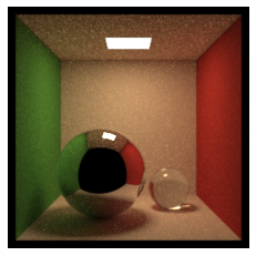
image = mi.render(scene, spp=256)
The render function returns the generated image as a tensor (mi.TensorXf, similar to a NumPy array) in linear RGB color space. The tensor class interfaces seamlessly with functions expecting NumPy arrays. For example, we can display the image using matplotlib.
[6]:
import matplotlib.pyplot as plt

plt.axis("off")
plt.imshow(image ** (1.0 / 2.2)); # approximate sRGB tonemapping
Clipping input data to the valid range for imshow with RGB data ([0..1] for floats or [0..255] for integers).
Writing an image to file
The mi.util.write_bitmap() function allows to save an image to disk and supports multiple file formats. If a low dynamic range (LDR) format is selected (e.g., PNG), this function tonemaps the image to the sRGB color space before saving.
[7]:
mi.util.write_bitmap("my_first_render.png", image)
mi.util.write_bitmap("my_first_render.exr", image)
Bravo! 🎉 You have now successfully rendered your first image!